Developing a placental epigenetic risk score for maternal BMI
By Meredith Palmore, epigenetic risk score adapted from Ellen Howerton
Background
Maternal body mass index (BMI) is a known risk factor of child health outcomes, such as childhood obesity, preterm birth, and infant mortality. Additionally, the theory of biological embedding highlights that early life conditions, such as those conferred by maternal BMI, may contribute to healthfulness of offspring later in life. Despite the correlational evidence behind the impacts of maternal BMI on child health outcomes, fewer studies have examined the biological pathways linking maternal education to child health outcomes. There is a clear need to examine how biological pathways related to maternal prepregnancy BMI may contribute to later child health.
A plausible biological mechanism is epigenetic alterations to the placenta. The placenta mediates the transfer of life-supporting nutrients and stress signals to the developing fetus. Changes to the placental epigenome in the form of DNA methylation impact gene regulation and could serve as a biological mechanism for adverse infant health outcomes related to exposures during pregnancy. Both candidate gene studies and epigenome wide association studies (EWAS) have revealed relationships between maternal pre-pregnancy BMI and DNA methylation changes in the newborn epigenome. In this analysis, I aim to summarize the impact of maternal BMI on the fetal side of the placental epigenome in an epigenetic risk score. Capturing alterations to the infant epigenome during pregnancy in an epigenetic risk score will help to improve our understanding of the relationship between maternal BMI and adverse infant health outcomes. Understanding the biological risk of maternal BMI on infant health may influence the prioritization of public health initiatives and policies that target maternal health.
Description:
The primary goal of this analysis is to summarize the relationship between the infant epigenome and maternal BMI in a weighted epigenetic risk score. Predictors of epigenetic risk will be derived from summary statistics of a previous EWAS of pre-pregnancy BMI on placental DNA methylation. Epigenetic risk score performance will be validated in the RICHS cohort.
This function and following code show the DNA methylation scoring procedure for difference in M-value in placental tissue, comparing mothers with different BMI categories. The main scoring procedure is in the function, and then after all scoring is completed, the performance is evaluated and the results are plotted.
Some notes on the epigenetic risk score:
One of my colleagues, Ellen Howerton, kindly provided me with the function for the epigenetic risk score. I have modified it to work with categorical variables with multiple levels.
toppg_11 are the summary statistics derived from limma’s topTable() (rownames are CpG sites, column names are effect size of logFC, P.Value, etc.)
The M-value matrix, or the individual-level methylation data matrix, in this example is named M_regress
absmeans are the average of the absolute value of effect sizes.
Here, I have included one variable to score, BMI category, as well as scoring by p-value threshold, but it could be modified to be multiple variables and a CpG list to be more generalizable.
Wrangling the Data
Part 1. Load packages
library(tidyverse)
library(data.table)
library(reshape2)
library(here)

if (!requireNamespace("BiocManager", quietly = TRUE))
  install.packages("BiocManager")

#BiocManager::install("IlluminaHumanMethylation450kanno.ilmn12.hg19")

library(IlluminaHumanMethylation450kanno.ilmn12.hg19)
library(methyland) #A package for imputation that I made myself! It requires the Annotation file loaded above.
library(fmsb)
library(pROC)
library(readxl)
Part 2. Load in my M-value matrix and summary statistics
A couple of notes about the methylation data:
Here is a link to the study from which I derived summary statistics: https://pubmed.ncbi.nlm.nih.gov/32071425/
Here is a link to the study where I derived my GEO dataset: http://dx.doi.org/10.1080/15592294.2016.1195534
The summary statistics were derived from linear models adjusted for surrogate variables as proxy for placenta cellular heterogeneity, SNP-based ancestry principal components, methylation principal components, maternal age, race and ethnicity, offspring sex,and sequencing batches.
Both the summary statistics and methylation data are measured from placental tissue on the 450K methylation array.
Now I will load in the summary data for our risk score algorithm. There are multiple files for the summary statistics because they were converted from a pdf file.
#My top_11 frame (it's not a limma object, it's loaded in as a .csv)

setwd("C:/Users/softb/OneDrive - Johns Hopkins/Thesis/Data/Summ_stats_BMI/")

temp = list.files(pattern="*.csv")
myfiles = lapply(temp, read.csv)

for(i in 1:length(myfiles)){colnames(myfiles[[i]]) <- c("CpGs", "chrom", "logFC", "p-value", "direction")}


top_11 <- myfiles %>% bind_rows()

head(top_11)
        CpGs chrom        logFC   p-value     direction
1 cg10143030  chr2  0.004584571 0.2115875 Hypermethylat
2 cg07848601  chr5  0.009093954 0.2151436 Hypermethylat
3 cg26466094  chr1 -0.007766493 0.2162056  Hypomethylat
4 cg16724319  chr2 -0.050483370 0.2181015  Hypomethylat
5 cg22197787  chr1 -0.003223481 0.2339715  Hypomethylat
6 cg13266327  chr2  0.004322822 0.2374356 Hypermethylat
top_11 <- as_tibble(top_11)
# Any missing data?
pMiss <- function(x){sum(is.na(x))/length(x)*100}
apply(top_11,2,pMiss)
      CpGs      chrom      logFC    p-value  direction
0.00000000 0.00000000 0.05307856 0.00000000 0.00000000
# One logFC value missing, so I will remove it.
top_11 <- top_11[-c(which(is.na(top_11$logFC))),]
# Make all of the columns numeric:
colnames(top_11)
[1] "CpGs" "chrom" "logFC" "p-value" "direction"top_11$logFC <- as.numeric(top_11$logFC)
top_11$`p-value` <- as.numeric(top_11$`p-value`)
Now, I will load in the methylation data. We expect to see a data-frame with 237 subjects (columns) and a bit fewer than 450K rows of data corresponding to the CpG probes.
## My M-matrix:

setwd("C:/Users/softb/OneDrive - Johns Hopkins/Thesis/Data")
load("Mval_Matrix.rda")

dim(M_regress)
[1] 336484 237Part 3. Subset matrix to probes that transfer from the EPIC to 450K array
The methylation matrix from GEO is already cleaned. However, during the cleaning process, the authors filtered out many probes, inclusing ones with little variability in methylation. I need some of the probes that they filtered out.
There are two possible ways that I will deal with the probes that do not transfer: Either…
drop them from the analysis
find the nearest probes that we have measured and retain those for the score
I will try option 2. I wrote a function that will find the nearest probe for which we have methylation data measured, and return a list of those probes.
I developed an imputation function that finds the nearest probe on the array that is also in our dataset.
# # Option 2: Substitute missing with an imputation function I developed
      missing_fromMatrix <- top_11[which(!top_11$CpGs %in% rownames(M_regress)), 1]
      missing_fromMatrix <- deframe(missing_fromMatrix)
      closest_probe <- findSub(missing_fromMatrix, M_regress, annotation= "Illumina450k")

      closest_probe[,1] %in% rownames(M_regress)
  [1] TRUE TRUE TRUE TRUE TRUE TRUE TRUE TRUE TRUE TRUE TRUE TRUE TRUE
 [14] TRUE TRUE TRUE TRUE TRUE TRUE TRUE TRUE TRUE TRUE TRUE TRUE TRUE
 [27] TRUE TRUE TRUE TRUE TRUE TRUE TRUE TRUE TRUE TRUE TRUE TRUE TRUE
 [40] TRUE TRUE TRUE TRUE TRUE TRUE TRUE TRUE TRUE TRUE TRUE TRUE TRUE
 [53] TRUE TRUE TRUE TRUE TRUE TRUE TRUE TRUE TRUE TRUE TRUE TRUE TRUE
 [66] TRUE TRUE TRUE TRUE TRUE TRUE TRUE TRUE TRUE TRUE TRUE TRUE TRUE
 [79] TRUE TRUE TRUE TRUE TRUE TRUE TRUE TRUE TRUE TRUE TRUE TRUE TRUE
 [92] TRUE TRUE TRUE TRUE TRUE TRUE TRUE TRUE TRUE TRUE TRUE TRUE TRUE
[105] TRUE TRUE TRUE TRUE TRUE TRUE TRUE TRUE
# All TRUE! :)
# The first column are the probes that were substituted, the second is the nearest probe that my imputation function found. The third column is the distance between the two probes in base-pairs.
head(closest_probe)
           Nearest_Probe Distance
cg13266327 "cg03997139"  "9"
cg03393966 "cg10740054"  "11"
cg15119377 "cg03518058"  "82"
cg20227592 "cg13902024"  "25384"
cg10442251 "cg23010629"  "22"
cg07708472 "cg19807612"  "50"
# Subset M-matrix to these probes (all 50)
index_scoreprobes <- which(rownames(M_regress) %in% top_11$CpGs)
index_imputedprobes <- which(rownames(M_regress) %in% closest_probe[,1])
index_allprobes <- c(index_scoreprobes, index_imputedprobes)
M_regress <- M_regress[index_allprobes,]
#rename the substituted probes in the toptable
closest_probe <- tibble::rownames_to_column(as.data.frame(closest_probe), "CpGs")
top_11 <- left_join(top_11, closest_probe, by="CpGs")
top_11 <- top_11 %>% mutate(CpGs = ifelse(is.na(Nearest_Probe), CpGs, Nearest_Probe))
top_11 %>% select(CpGs, Nearest_Probe)
# A tibble: 1,883 x 2
   CpGs       Nearest_Probe
   <chr>      <chr>
 1 cg10143030 <NA>
 2 cg07848601 <NA>
 3 cg26466094 <NA>
 4 cg16724319 <NA>
 5 cg22197787 <NA>
 6 cg03997139 cg03997139
 7 cg10740054 cg10740054
 8 cg20594982 <NA>
 9 cg05638699 <NA>
10 cg16274199 <NA>
# ... with 1,873 more rows[1] FALSE top_11<- top_11 %>% filter(duplicated(CpGs) == FALSE)
#Will keep the true (non-imputed) CpG because it has a stronger association and is located closer to the top of the list
Now that we have imputed the missing probes with nearby ones and updated them in the methylation matrix and in the top_11 object (summary statistics object), we can proceed with our computation of the score.
For the score, we must find the average absolute value of the logFC, or the log-fold change in methylation for each unit increase in BMI, and save it for later:
top_11$logFC <- as.numeric(top_11$logFC)
  absmean_pg_11 <- mean(abs(top_11$logFC))
  absmean_pg_11
[1] 0.005470551Part 4. Select individuals with phenotype information
The sample annotation file contains all the phenotypic data of the subjects in the RICHS cohort. We would expect that the rows in the phenotypic dataset correspond perfectly to the columns in the methylation dataset. Here, I will only retain the sample IDs and the outcome of interest, BMI.
Then, I calculate BMI categories because I need to be able to specify a reference group that I will compare mean methylation levels to, namely individuals with “normal” BMIs.
# Load in phenotype information

load("C:/Users/softb/OneDrive - Johns Hopkins/Thesis/Data/Subset_Annotation.rda")

pd <- subset_anno %>%
  mutate("SampleID" = geo_accession, .before = geo_accession) %>%
  select(SampleID, bmi)

#We expect to have 237 rows of data, corresponding with the 237 columns in the

head(pd)
             SampleID      bmi
GSM1947017 GSM1947017 39.91943
GSM1947018 GSM1947018 44.05074
GSM1947019 GSM1947019 19.60968
GSM1947020 GSM1947020 28.56811
GSM1947021 GSM1947021 21.31254
GSM1947023 GSM1947023 39.16633dim(pd)
[1] 237 2# Is there any missing data?
apply(pd,2,pMiss) # No.
SampleID      bmi
       0        0
# Divide BMI into categories.
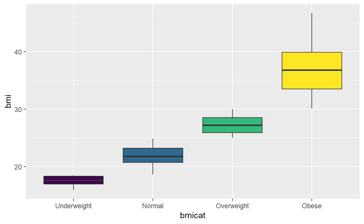
pd$bmi <- as.numeric(pd$bmi)
pd = dplyr::mutate(pd, bmicat = cut(bmi, breaks = c(0,18.5, 25, 30,100), labels = 1:4, ordered = TRUE))
ggplot(pd, aes(bmicat, bmi, fill = bmicat)) +
geom_boxplot() +
scale_x_discrete(labels=c("1" = "Underweight", "2" = "Normal",
"3" = "Overweight", "4" = "Obese"))+
theme(legend.position= "none")
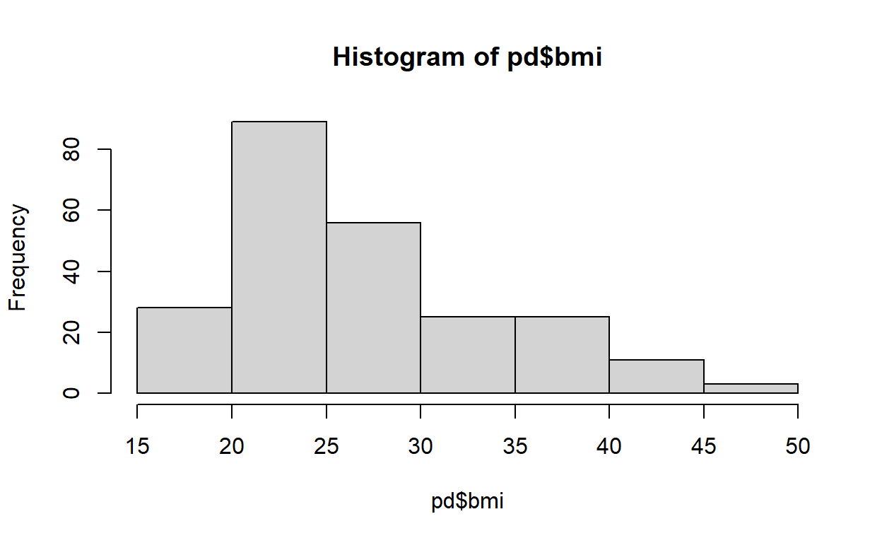
hist(pd$bmi) #Very right skewed
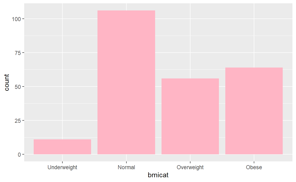
ggplot(pd, aes(bmicat)) +
  geom_histogram(stat="count", fill = "pink1") +
  scale_x_discrete(labels=c("1" = "Underweight", "2" = "Normal",
                              "3" = "Overweight", "4" = "Obese"))
class(pd$bmicat)
[1] "ordered" "factor" #Make sure there are 237 subjects in the sample annotation and the methylation data files.
dim(M_regress)
[1] 1869 237dim(pd)
[1] 237 3Run the epigenetic risk score function
Since the outcome is not binary, the baseline we are standardizing our methylation levels to are individuals with ‘normal’ BMI. So when comparing methylation to the the median value of the “unexposed”, the unexposed is individuals with normal BMI.
score_ts_byM_p <- function(variable, pthresh) {

  top_11 <- top_11[top_11$`p-value` <= pthresh,]
  top_11 <- mutate(top_11, CpG_site = CpGs)

  top_11 <- top_11 %>%
    as_tibble() %>%
    dplyr::mutate(CpG_site = as.factor(CpG_site))

  if(nrow(top_11) == 0) {
    print(paste0("There are no CpGs that reached significance for p <= ", pthresh, ". Stopping function."))
    stop()
  }

  print(paste0("Here are the CpG sites that have a p-value <=  ", pthresh, ":"))
  print(top_11)
  fwrite(top_11, file.path("projects_files", paste0("cpg_list_in_score_", pthresh, "_", variable, ".csv")))

  # prep count name
  count_name <- paste0("count_", pthresh)

  top_count_t_11 <- top_11 %>%
     as_tibble() %>%
     dplyr::mutate(CpG_site = as.factor(CpG_site)) %>%
    dplyr::summarise(!!count_name := n(), total_CpGs = nrow(top_11))
  print(top_count_t_11)
  fwrite(top_count_t_11,file.path("projects_files",paste0("cpg_count_in_score_", pthresh, "_", variable, ".csv")))
  # Note: Had to remove the directory specified because I don't have it.

  # subset M-value matrix
  t_cpg_site_names <- top_11 %>%
    dplyr::select(CpG_site) %>%
    dplyr::mutate(CpG_site = as.character(CpG_site)) %>%
    deframe()

  M_11 <- M_regress[t_cpg_site_names,] %>%
    t() %>%
    as.data.frame()
  print("The dimensions of the M-value object, subsetted by CpG sites of interest:")
   #print(head(M_11))
   #print(tail(M_11))
  print(dim(M_11))

  # bind phenotype information
  M_inf_11 <- cbind(M_11, pd[ ,c("SampleID","bmicat")])
  print("The dimensions of the M-value object, with bmi information:")
   #print(head(M_inf_11))
   #print(tail(M_inf_11))
  print(dim(M_inf_11))

  M_inf_11 <- M_inf_11 %>%
    dplyr::as_tibble()

  #print("dimensions of the tibble:")
  #print(dim(M_inf_11))

  # reshape data to long
  M_inf_melt_11 <- M_inf_11 %>%
    #dplyr::as_tibble() %>%
    melt(id.vars = c("SampleID","bmicat")) %>%
    #dplyr::as_tibble() %>%
    dplyr::rename(CpG_site = variable) %>%
    dplyr::rename(M_value = value)

  top_11$CpG_site <- as.character(top_11$CpG_site)
  M_inf_melt_11$CpG_site <- as.character(M_inf_melt_11$CpG_site)

  M_inf_melt_11 <- M_inf_melt_11 %>%
    dplyr::left_join(top_11, by = "CpG_site")

  print("The 'melted' M-value object, with bmi information:")
  print(summary(M_inf_melt_11))


  # empty median M value tibble
  med_M <- tibble(CpG_site = factor(),
                  #timeframe = factor(),
                  med_M_unexp = numeric())
  print("Check (empty) median M value tibble:")
  print(med_M)


  # for loop to add in median M value for the reference group (normal BMI = 2) for each CpG and time period


  pd$bmicat <- as.numeric(pd$bmicat)

  top_11$CpG_site <- as.factor(top_11$CpG_site)

  for(i in seq_along(levels(top_11$CpG_site))) {

    i_nm <- top_11$CpG_site[[i]]

       row_M <- M_inf_melt_11 %>%
         dplyr::mutate(CpG_site = as.factor(CpG_site)) %>%
         dplyr::filter(CpG_site == i_nm & bmicat == 2) %>%
         dplyr::summarize(CpG_site, med_M_unexp = median(M_value)) %>%
         distinct()
       med_M <- bind_rows(med_M, row_M)
  }

   print("Here is the median M-value of normal BMI (reference group) for all CpGs in the score:")
   print(med_M)

  # join the median unexposed to the melt score object
  M_inf_melt_med <- dplyr::left_join(M_inf_melt_11, med_M, by = "CpG_site")
  # print(M_inf_melt_med)

  print("Check that median values joined correctly:")
  print(summary(M_inf_melt_med))

  # prep names for score columns
  score_name <- paste0("score_", pthresh)
  score_name <- gsub("e-", "E_", score_name)

  # score!
  M_inf_melt_score <- M_inf_melt_med %>%
    dplyr::mutate(score_cpg  = (logFC / absmean_pg_11) * (M_value - med_M_unexp)) %>%
    dplyr::group_by(SampleID) %>%
    dplyr::mutate(!!score_name := sum(score_cpg))

  print(paste0("Scores are complete for the variable: ", variable, " and the p-value threshold of: ", pthresh))

  # make more mergeable
  M_inf_melt_score %>%
    dplyr::select(SampleID, bmicat, !!score_name) %>%
    distinct()

}
Results
Part 1. Make functions for results tables and graphs
Now that we have computed the scores, we can make functions for the results that include figures and regression results.
Functions make my code look nicer and more concise to have graphs summarizing the results from the risk score calculations.
gress_graph <- function(score){

  indv_scores <- as.matrix(score[,3])

  score$bmicat <- factor(score$bmicat, ordered = FALSE)
  score$bmicat <- relevel(score$bmicat, ref = 2)

  mod <- lm(indv_scores ~ bmicat, data = score)
  mean_change <- coef(mod)
  conf <- confint(mod)
  print(mean_change)
  print(conf)
  print(summary(mod)$r.squared)
  print(aic(mod))


   ggplot(score, aes(x = bmicat, y = indv_scores)) +
     geom_violin(fill = "pink1") +
     geom_point(alpha=0.5) +
     scale_x_discrete(labels=c("1" = "Underweight", "2" = "Normal",
                              "3" = "Overweight", "4" = "Obese"))

}
Part 2. Display the results
M_score_pg_1E_03 <- score_ts_byM_p("bmicat", 1*10^-3)
[1] "Here are the CpG sites that have a p-value <=  0.001:"
# A tibble: 2 x 8
  CpGs       chrom    logFC `p-value` direction Nearest_Probe Distance
  <chr>      <chr>    <dbl>     <dbl> <chr>     <chr>         <chr>
1 cg13014558 chr11 -0.00603  0.000503 Hypometh~ <NA>          <NA>
2 cg26947572 chr2  -0.0118   0.000723 Hypometh~ <NA>          <NA>
# ... with 1 more variable: CpG_site <fct>
# A tibble: 1 x 2
  count_0.001 total_CpGs
        <int>      <int>
1           2          2
[1] "The dimensions of the M-value object, subsetted by CpG sites of interest:"
[1] 237   2
[1] "The dimensions of the M-value object, with bmi information:"
[1] 237   4
[1] "The 'melted' M-value object, with bmi information:"
   SampleID         bmicat    CpG_site            M_value
 Length:474         1: 22   Length:474         Min.   :-6.02212
 Class :character   2:212   Class :character   1st Qu.:-5.17617
 Mode  :character   3:112   Mode  :character   Median :-2.33216
                    4:128                      Mean   :-2.53902
                                               3rd Qu.: 0.09552
                                               Max.   : 0.59106
     CpGs              chrom               logFC
 Length:474         Length:474         Min.   :-0.011773
 Class :character   Class :character   1st Qu.:-0.011773
 Mode  :character   Mode  :character   Median :-0.008900
                                       Mean   :-0.008900
                                       3rd Qu.:-0.006027
                                       Max.   :-0.006027
    p-value           direction         Nearest_Probe
 Min.   :0.0005027   Length:474         Length:474
 1st Qu.:0.0005027   Class :character   Class :character
 Median :0.0006129   Mode  :character   Mode  :character
 Mean   :0.0006129
 3rd Qu.:0.0007231
 Max.   :0.0007231
   Distance
 Length:474
 Class :character
 Mode  :character


[1] "Check (empty) median M value tibble:"
# A tibble: 0 x 2
# ... with 2 variables: CpG_site <fct>, med_M_unexp <dbl>
[1] "Here is the median M-value of normal BMI (reference group) for all CpGs in the score:"
# A tibble: 2 x 2
  CpG_site   med_M_unexp
  <fct>            <dbl>
1 cg13014558      0.0825
2 cg26947572     -5.20
[1] "Check that median values joined correctly:"
   SampleID         bmicat    CpG_site            M_value
 Length:474         1: 22   Length:474         Min.   :-6.02212
 Class :character   2:212   Class :character   1st Qu.:-5.17617
 Mode  :character   3:112   Mode  :character   Median :-2.33216
                    4:128                      Mean   :-2.53902
                                               3rd Qu.: 0.09552
                                               Max.   : 0.59106
     CpGs              chrom               logFC
 Length:474         Length:474         Min.   :-0.011773
 Class :character   Class :character   1st Qu.:-0.011773
 Mode  :character   Mode  :character   Median :-0.008900
                                       Mean   :-0.008900
                                       3rd Qu.:-0.006027
                                       Max.   :-0.006027
    p-value           direction         Nearest_Probe
 Min.   :0.0005027   Length:474         Length:474
 1st Qu.:0.0005027   Class :character   Class :character
 Median :0.0006129   Mode  :character   Mode  :character
 Mean   :0.0006129
 3rd Qu.:0.0007231
 Max.   :0.0007231
   Distance          med_M_unexp
 Length:474         Min.   :-5.19757
 Class :character   1st Qu.:-5.19757
 Mode  :character   Median :-2.55752
                    Mean   :-2.55752
                    3rd Qu.: 0.08254
                    Max.   : 0.08254
[1] "Scores are complete for the variable: bmicat and the p-value threshold of: 0.001" gress_graph(M_score_pg_1E_03)
(Intercept)     bmicat1     bmicat3     bmicat4
-0.02918356  0.08305977 -0.18809819  0.00519048
                 2.5 %      97.5 %
(Intercept) -0.1443039 0.085936813
bmicat1     -0.2923874 0.458506904
bmicat3     -0.3838995 0.007703169
bmicat4     -0.1824328 0.192813739
[1] 0.01970488
       lik       infl       vari        aic
-42.185102 3.433483 3.336728 91.237169 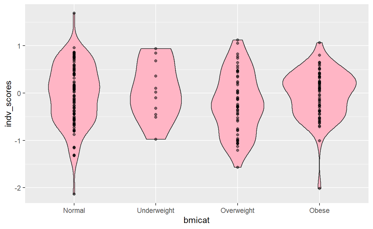
M_score_pg_1E_02 <- score_ts_byM_p("bmicat", 1*10^-2)
[1] "Here are the CpG sites that have a p-value <=  0.01:"
# A tibble: 53 x 8
   CpGs     chrom    logFC `p-value` direction  Nearest_Probe Distance
   <chr>    <chr>    <dbl>     <dbl> <chr>      <chr>         <chr>
 1 cg13014~ chr11 -0.00603  0.000503 Hypomethy~ <NA>          <NA>
 2 cg26947~ chr2  -0.0118   0.000723 Hypomethy~ <NA>          <NA>
 3 cg05633~ chr2   0.0493   0.00108  Hypermeth~ <NA>          <NA>
 4 cg01054~ chr12  0.00608  0.00113  Hypermeth~ <NA>          <NA>
 5 cg12902~ chr1  -0.0327   0.00123  Hypomethy~ <NA>          <NA>
 6 cg11428~ chr22  0.0128   0.00157  Hypermeth~ <NA>          <NA>
 7 cg03719~ chr20 -0.0115   0.00160  Hypomethy~ <NA>          <NA>
 8 cg17492~ chr2  -0.0210   0.00167  Hypomethy~ <NA>          <NA>
 9 cg13782~ chr14 -0.0133   0.00170  Hypomethy~ <NA>          <NA>
10 cg02759~ chr4  -0.0682   0.00172  Hypomethy~ <NA>          <NA>
# ... with 43 more rows, and 1 more variable: CpG_site <fct>
# A tibble: 1 x 2
  count_0.01 total_CpGs
       <int>      <int>
1         53         53
[1] "The dimensions of the M-value object, subsetted by CpG sites of interest:"
[1] 237  53
[1] "The dimensions of the M-value object, with bmi information:"
[1] 237  55
[1] "The 'melted' M-value object, with bmi information:"
   SampleID         bmicat     CpG_site            M_value
 Length:12561       1: 583   Length:12561       Min.   :-8.691
 Class :character   2:5618   Class :character   1st Qu.:-5.480
 Mode  :character   3:2968   Mode  :character   Median :-4.998
                    4:3392                      Mean   :-3.688
                                                3rd Qu.:-2.463
                                                Max.   : 5.809
     CpGs              chrom               logFC
 Length:12561       Length:12561       Min.   :-0.068234
 Class :character   Class :character   1st Qu.:-0.014400
 Mode  :character   Mode  :character   Median :-0.011544
                                       Mean   :-0.004837
                                       3rd Qu.: 0.008676
                                       Max.   : 0.050861
    p-value           direction         Nearest_Probe
 Min.   :0.0005027   Length:12561       Length:12561
 1st Qu.:0.0021486   Class :character   Class :character
 Median :0.0037328   Mode  :character   Mode  :character
 Mean   :0.0044511
 3rd Qu.:0.0066821
 Max.   :0.0095655
   Distance
 Length:12561
 Class :character
 Mode  :character


[1] "Check (empty) median M value tibble:"
# A tibble: 0 x 2
# ... with 2 variables: CpG_site <fct>, med_M_unexp <dbl>
[1] "Here is the median M-value of normal BMI (reference group) for all CpGs in the score:"
# A tibble: 53 x 2
   CpG_site   med_M_unexp
   <fct>            <dbl>
 1 cg13014558      0.0825
 2 cg26947572     -5.20
 3 cg05633391     -5.41
 4 cg01054110      1.95
 5 cg12902497     -5.66
 6 cg11428482     -5.59
 7 cg03719642      2.19
 8 cg17492041     -5.40
 9 cg13782781     -5.06
10 cg02759110     -4.22
# ... with 43 more rows
[1] "Check that median values joined correctly:"
   SampleID         bmicat     CpG_site            M_value
 Length:12561       1: 583   Length:12561       Min.   :-8.691
 Class :character   2:5618   Class :character   1st Qu.:-5.480
 Mode  :character   3:2968   Mode  :character   Median :-4.998
                    4:3392                      Mean   :-3.688
                                                3rd Qu.:-2.463
                                                Max.   : 5.809
     CpGs              chrom               logFC
 Length:12561       Length:12561       Min.   :-0.068234
 Class :character   Class :character   1st Qu.:-0.014400
 Mode  :character   Mode  :character   Median :-0.011544
                                       Mean   :-0.004837
                                       3rd Qu.: 0.008676
                                       Max.   : 0.050861
    p-value           direction         Nearest_Probe
 Min.   :0.0005027   Length:12561       Length:12561
 1st Qu.:0.0021486   Class :character   Class :character
 Median :0.0037328   Mode  :character   Mode  :character
 Mean   :0.0044511
 3rd Qu.:0.0066821
 Max.   :0.0095655
   Distance          med_M_unexp
 Length:12561       Min.   :-6.278
 Class :character   1st Qu.:-5.427
 Mode  :character   Median :-5.071
                    Mean   :-3.704
                    3rd Qu.:-2.424
                    Max.   : 5.042
[1] "Scores are complete for the variable: bmicat and the p-value threshold of: 0.01" gress_graph(M_score_pg_1E_02)
(Intercept)     bmicat1     bmicat3     bmicat4
  -5.477925    2.052503    2.507837    3.408030
                 2.5 %     97.5 %
(Intercept)  -9.974812 -0.9810378
bmicat1     -12.613392 16.7183980
bmicat3      -5.140650 10.1563227
bmicat4      -3.920999 10.7370597
[1] 0.004094288
          lik          infl          vari           aic
-64335.112821 3.433483 3.336728 128677.092608 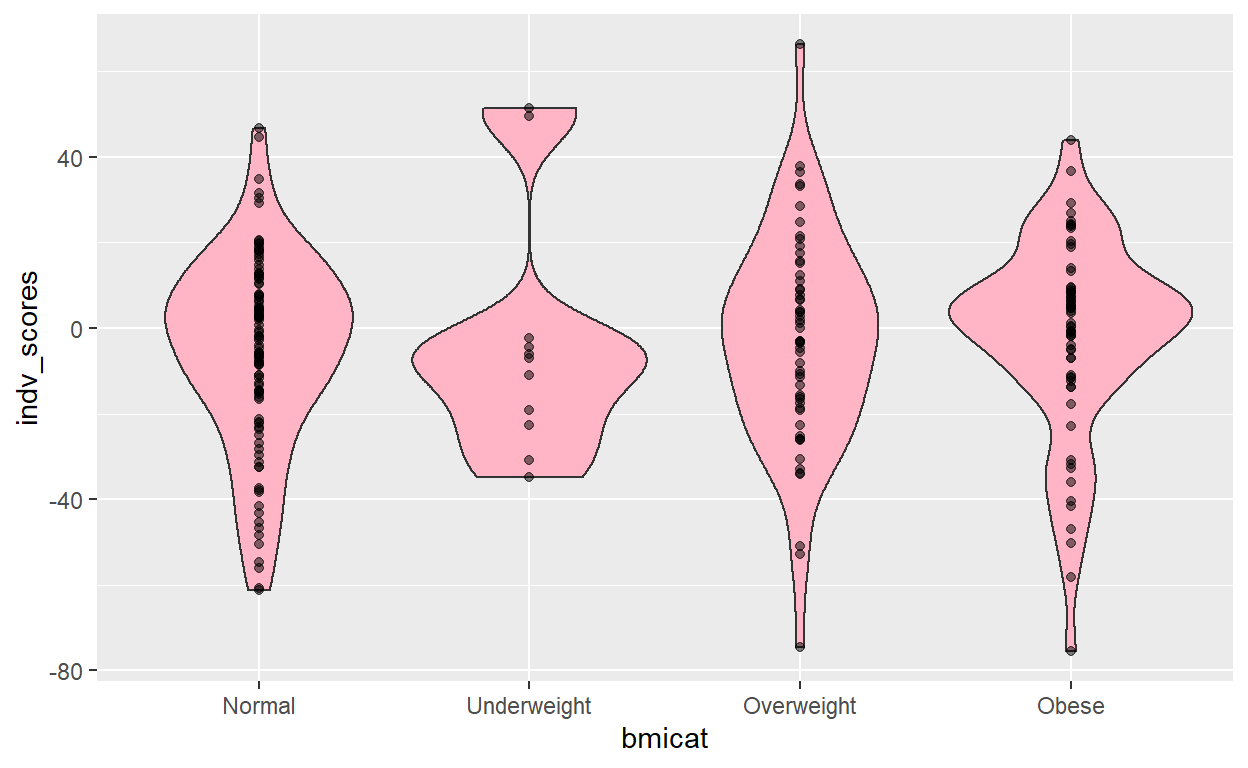
M_score_pg_1E_01 <- score_ts_byM_p("bmicat", 1*10^-1)
[1] "Here are the CpG sites that have a p-value <=  0.1:"
# A tibble: 312 x 8
   CpGs     chrom    logFC `p-value` direction  Nearest_Probe Distance
   <chr>    <chr>    <dbl>     <dbl> <chr>      <chr>         <chr>
 1 cg13014~ chr11 -0.00603  0.000503 Hypomethy~ <NA>          <NA>
 2 cg26947~ chr2  -0.0118   0.000723 Hypomethy~ <NA>          <NA>
 3 cg05633~ chr2   0.0493   0.00108  Hypermeth~ <NA>          <NA>
 4 cg01054~ chr12  0.00608  0.00113  Hypermeth~ <NA>          <NA>
 5 cg12902~ chr1  -0.0327   0.00123  Hypomethy~ <NA>          <NA>
 6 cg11428~ chr22  0.0128   0.00157  Hypermeth~ <NA>          <NA>
 7 cg03719~ chr20 -0.0115   0.00160  Hypomethy~ <NA>          <NA>
 8 cg17492~ chr2  -0.0210   0.00167  Hypomethy~ <NA>          <NA>
 9 cg13782~ chr14 -0.0133   0.00170  Hypomethy~ <NA>          <NA>
10 cg02759~ chr4  -0.0682   0.00172  Hypomethy~ <NA>          <NA>
# ... with 302 more rows, and 1 more variable: CpG_site <fct>
# A tibble: 1 x 2
  count_0.1 total_CpGs
      <int>      <int>
1       312        312
[1] "The dimensions of the M-value object, subsetted by CpG sites of interest:"
[1] 237 312
[1] "The dimensions of the M-value object, with bmi information:"
[1] 237 314
[1] "The 'melted' M-value object, with bmi information:"
   SampleID         bmicat      CpG_site            M_value
 Length:73944       1: 3432   Length:73944       Min.   :-9.173
 Class :character   2:33072   Class :character   1st Qu.:-5.479
 Mode  :character   3:17472   Mode  :character   Median :-5.011
                    4:19968                      Mean   :-3.316
                                                 3rd Qu.:-1.815
                                                 Max.   : 6.834
     CpGs              chrom               logFC
 Length:73944       Length:73944       Min.   :-0.068234
 Class :character   Class :character   1st Qu.:-0.011853
 Mode  :character   Mode  :character   Median :-0.007394
                                       Mean   :-0.003419
                                       3rd Qu.: 0.007900
                                       Max.   : 0.050861
    p-value           direction         Nearest_Probe
 Min.   :0.0005027   Length:73944       Length:73944
 1st Qu.:0.0168901   Class :character   Class :character
 Median :0.0394770   Mode  :character   Mode  :character
 Mean   :0.0439951
 3rd Qu.:0.0709698
 Max.   :0.0995257
   Distance
 Length:73944
 Class :character
 Mode  :character


[1] "Check (empty) median M value tibble:"
# A tibble: 0 x 2
# ... with 2 variables: CpG_site <fct>, med_M_unexp <dbl>
[1] "Here is the median M-value of normal BMI (reference group) for all CpGs in the score:"
# A tibble: 312 x 2
   CpG_site   med_M_unexp
   <fct>            <dbl>
 1 cg13014558      0.0825
 2 cg26947572     -5.20
 3 cg05633391     -5.41
 4 cg01054110      1.95
 5 cg12902497     -5.66
 6 cg11428482     -5.59
 7 cg03719642      2.19
 8 cg17492041     -5.40
 9 cg13782781     -5.06
10 cg02759110     -4.22
# ... with 302 more rows
[1] "Check that median values joined correctly:"
   SampleID         bmicat      CpG_site            M_value
 Length:73944       1: 3432   Length:73944       Min.   :-9.173
 Class :character   2:33072   Class :character   1st Qu.:-5.479
 Mode  :character   3:17472   Mode  :character   Median :-5.011
                    4:19968                      Mean   :-3.316
                                                 3rd Qu.:-1.815
                                                 Max.   : 6.834
     CpGs              chrom               logFC
 Length:73944       Length:73944       Min.   :-0.068234
 Class :character   Class :character   1st Qu.:-0.011853
 Mode  :character   Mode  :character   Median :-0.007394
                                       Mean   :-0.003419
                                       3rd Qu.: 0.007900
                                       Max.   : 0.050861
    p-value           direction         Nearest_Probe
 Min.   :0.0005027   Length:73944       Length:73944
 1st Qu.:0.0168901   Class :character   Class :character
 Median :0.0394770   Mode  :character   Mode  :character
 Mean   :0.0439951
 3rd Qu.:0.0709698
 Max.   :0.0995257
   Distance          med_M_unexp
 Length:73944       Min.   :-6.368
 Class :character   1st Qu.:-5.468
 Mode  :character   Median :-5.087
                    Mean   :-3.312
                    3rd Qu.:-1.914
                    Max.   : 5.611
[1] "Scores are complete for the variable: bmicat and the p-value threshold of: 0.1" gress_graph(M_score_pg_1E_01)
(Intercept)     bmicat1     bmicat3     bmicat4
  -8.293362    6.441864    2.134842    2.712726
                2.5 %    97.5 %
(Intercept) -17.08768  0.500951
bmicat1     -22.23942 35.123144
bmicat3     -12.82288 17.092563
bmicat4     -11.62025 17.045704
[1] 0.001265498
          lik          infl          vari           aic
-2.460468e+05 3.433483e+00 3.336728e+00 4.921005e+05 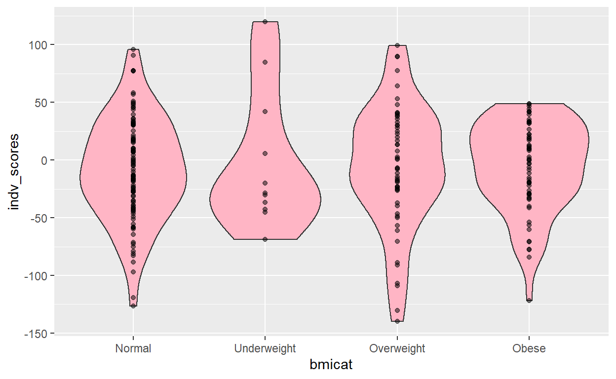
Discussion of the results
The model with the most stringent pruning threshold has the best discrimination, with an \(R^{2}\) of 2.0%. Additionally, since only 2 methylation loci were included, it was the most parsimonious model as well, with an AIC of just 91.24.
Additionally, the effect estimates are credible. Children with mothers with “normal” and “overweight” BMIs have comparable slight decrease in epigenetic risk scores, whereas those who were underweight had highest risk and those who were obese had the second highest epigenetic risk scores. Perhaps there are common epigenome-wide changes in individuals in the upper and lower extremes of BMI. This might extend to help explain observations of greater risks to conception-related outcomes in women who are on the extremes: e.g. in underweight, such as low birth-weight and preterm birth, as well as the risks for obese women such as infant mortality and preterm birth (Cnattingius et al., 1998).
However, I will caution that these results are not to be taken as truth. The effect sizes are quite small and not significant, and this is not a rigorous study, just a project. Additionally, risk scores are not to be taken for causal inference and every individual is different. Individual level outcomes may not always reflect what you would predict based on population level data.
Limitations:
This was an exploratory analysis for a self-directed project. If I were doing a real study, I might consider addressing the following:
I did not adjust for confounding factors in the validation set, but the effect estimates included in the risk score itself should be un-confounded, assuming the study where the summary statistics came from properly accounted for confounding. I think this is a fair assumption. Their quality control procedures were quite comprehensive!
I did not account for global differences in methylation, only single site changes. The normalization steps in the publicly available studies may have diluted global changes. Additionally, if there were differences in global methylation levels that are related to differences in characteristics of the 2 populations, then I may have obtained biased results.
Since I used publicly available data, I am a bit unclear about the specifics of the measurement of BMI in these cohorts. Additionally, I cannot look at other relevant exposures such as weight gain during pregnancy, so I may be missing some important information.
Future perspectives:
Here are some guiding questions for projects that would help contextualize and improve my analysis:
How much does the epigenetic risk score explain independently when included in a model with other covariates?
How is the risk score associated with child health outcomes?
Behavioral Risk Factors of Excessive Daytime Sleepiness in NHANES 2017-18
Background
Insufficient sleep duration and quality is associated with both morbidity and mortality from cardiometabolic disorders and affects neurobehavioral functioning (Gangwesh at al., 2006; Hall et al., 2008).
The 20th century has seen a downward trend in sleep duration and quality (Bixler, 2009).
Studies have identified health behaviors and personal characteristics that contribute to shortened sleep duration, such as age, race, obesity, low physical activity, heavy alcohol use, high caffeine consumption, smoking (Bixler, 2009; Phillips, 1995; Temple et al., 2017; Schoenborn & Adams, 2019; Stein & Friedmann, 2005; Kredlow, 2015).
Few research studies have sought to identify whether these relationships hold when the outcome is sleep quality rather than duration.
Sleep quality may be different from sleep duration. The sleep cycle is complex and sleep duration is not always indicative of high-quality sleep. In addition, sufficient sleep duration may also vary depending on the individual (Bin, 2016).
Understanding factors associated with poor sleep quality could provide insight to actionable avenues for intervention and ultimately impact quality of life, and even morbidity and mortality.
Study Design
Data were obtained from National Health and Nutritional Examination Survey (NHANES) 2017-2018, a cross-sectional complex survey. Home interviews and exams were conducted on a nationally representative sample of adults and children in the United States. A population-based sample was derived from a complex multistage, probability sampling design. 9,254 participants were interviewed, and 8,704 were examined. Only participants aged 18 and older were included in the analysis, resulting in a study sample size of 5,856.
Data
Since this is a risk factor study, all exposures were considered equally with no primary exposure of interest. Potential risk factors were derived from evidence in the literature. BMI and caffeine intake were measured in the examination stage. Alcohol use, excessive daytime sleepiness, current smoking, depression score, race and ethnicity, age, and participation in moderate to vigorous exercise were all collected at the interview stage. All risk factors except for income-to-poverty ratio, were transformed into categorical variables based on literature-informed criteria and conventions.
Excessive daytime sleepiness was chosen as the outcome of interest. This outcome was selected over self-reported hours of sleep because it is an indicator of sleep quality, rather than sleep duration. The question asked to participants was “In the past month, how often did {you/survey participant} feel excessively or overly sleepy during the day?” Following the convention of Lal et al., participants responded as “Often” or “Almost always” were categorized as “Yes,” and other responses were categorized as “No. This study was exploratory in nature and meant to be hypothesis-generating and replicate prior associations between behavioral risk factors and sleep quality.
Wrangling the data
First, I will load in the packages that I will use for my analysis.
Now, I will read in my datasets. I exported the data from the NHANES 2018 website and converted them to .csv files. I will load them all and combine them into a larger file. I will merge all of the component files by the individuals’ identifying number (SEQN). I decide to left join with demography file as the leftmost column, because I want to retain the denominator of individuals even if some the predictor and outcome variables are missing.
temp = list.files(".","*.csv")
myfiles = lapply(temp, read.csv)

one_tmp <- myfiles[[5]] #This is the demographic dataset

for(i in c(1:4,6:8)){
  one_tmp <- left_join(one_tmp, myfiles[[i]], by = "SEQN")
}

# Fix the naming of some of these variables:

head(one_tmp)
  X.x  SEQN RIAGENDR RIDAGEYR RIDRETH3  WTINT2YR  WTMEC2YR SDMVPSU
1   1 93703        2        2        6  9246.492  8539.731       2
2   2 93704        1        2        3 37338.768 42566.615       1
3   3 93705        2       66        4  8614.571  8338.420       2
4   4 93706        1       18        6  8548.633  8723.440       2
5   5 93707        1       13        7  6769.345  7064.610       1
6   6 93708        2       66        6 13329.451 14372.489       2
  SDMVSTRA INDFMPIR X.y PAQ605 PAQ620 PAQ650 PAQ665 X.x.x ALQ111
1      145     5.00  NA     NA     NA     NA     NA    NA     NA
2      143     5.00  NA     NA     NA     NA     NA    NA     NA
3      145     0.82   1      2      2      2      1     1      1
4      134       NA   2      2      2      2      1     2      2
5      138     1.88  NA     NA     NA     NA     NA    NA     NA
6      138     1.63   3      2      2      2      1     3      2
  ALQ121 ALQ130 X.y.y BMXBMI X.x.x.x DR1TCAFF DR2TCAFF
1     NA     NA     1   17.5       1       NA       NA
2     NA     NA     2   15.7       2        8        6
3      7      1     3   31.7       3      361      146
4     NA     NA     4   21.5       4        0       NA
5     NA     NA     5   18.1       5       21       10
6     NA     NA     6   23.7       6       33        0
  avg_mg_caffeine X.y.y.y DPQ010 DPQ020 DPQ030 DPQ040 DPQ050 DPQ060
1              NA      NA     NA     NA     NA     NA     NA     NA
2             7.0      NA     NA     NA     NA     NA     NA     NA
3           253.5       1      0      0      0      0      0      0
4              NA       2      0      0      0      0      0      0
5            15.5      NA     NA     NA     NA     NA     NA     NA
6            16.5       3      0      0      0      0      0      0
  DPQ070 DPQ080 DPQ090 DPQ100 X.x.x.x.x SLD012 SLD013 SLQ120
1     NA     NA     NA     NA        NA     NA     NA     NA
2     NA     NA     NA     NA        NA     NA     NA     NA
3      0      0      0     NA         1    8.0    8.0      0
4      0      0      0     NA         2   10.5   11.5      1
5     NA     NA     NA     NA        NA     NA     NA     NA
6      0      0      0     NA         3    8.0    8.0      2
  day_sleep X.y.y.y.y SMQ681
1        NA        NA     NA
2        NA        NA     NA
3         0         1      2
4         0         2      2
5        NA         3      2
6 0 4 2# A tibble: 6 x 35
SEQN RIAGENDR RIDAGEYR RIDRETH3 WTINT2YR WTMEC2YR SDMVPSU SDMVSTRA
<dbl> <int> <int> <int> <dbl> <dbl> <int> <int>
1 93703 2 2 6 9246. 8540. 2 145
2 93704 1 2 3 37339. 42567. 1 143
3 93705 2 66 4 8615. 8338. 2 145
4 93706 1 18 6 8549. 8723. 2 134
5 93707 1 13 7 6769. 7065. 1 138
6 93708 2 66 6 13329. 14372. 2 138
# ... with 27 more variables: INDFMPIR <dbl>, PAQ605 <int>,
# PAQ620 <int>, PAQ650 <int>, PAQ665 <int>, ALQ111 <int>,
# ALQ121 <int>, ALQ130 <int>, BMXBMI <dbl>, DR1TCAFF <int>,
# DR2TCAFF <int>, avg_mg_caffeine <dbl>, DPQ010 <int>,
# DPQ020 <int>, DPQ030 <int>, DPQ040 <int>, DPQ050 <int>,
# DPQ060 <int>, DPQ070 <int>, DPQ080 <int>, DPQ090 <int>,
# DPQ100 <int>, SLD012 <dbl>, SLD013 <dbl>, SLQ120 <int>, ...# Worked beautifully!
Some of the data are labeled as numeric values if they were missing. Referring to NHANES documentation, you can see which numbers correspond to missing data, depending on the variable. It would be a good idea to convert them into simple NAs.
one_tmp <- one_tmp %>%
   mutate(across(starts_with('ALQ'), ~ case_when(. ==  77 ~ NA_integer_, . == 99 ~ NA_integer_, . == 777 ~ NA_integer_, . == 999 ~ NA_integer_, TRUE ~ as.integer(.))))


#For activity variables, change to missing if "Refused" or "Don't Know"

one_tmp <- one_tmp %>%
   mutate(across(starts_with('PAQ'), ~ case_when(. ==  9 ~ NA_integer_, TRUE ~ as.integer(.))))


#For depression variables, change to missing if "Refused" or "Don't Know"

one_tmp <- one_tmp %>%
   mutate(across(starts_with('DPQ'), ~ case_when(. ==  7 ~ NA_integer_, . ==  9 ~ NA_integer_, TRUE ~ as.integer(.))))

summary(one_tmp) # Looking better.
      SEQN           RIAGENDR        RIDAGEYR        RIDRETH3
 Min.   : 93703   Min.   :1.000   Min.   : 0.00   Min.   :1.000
 1st Qu.: 96016   1st Qu.:1.000   1st Qu.:11.00   1st Qu.:3.000
 Median : 98330   Median :2.000   Median :31.00   Median :3.000
 Mean   : 98330   Mean   :1.508   Mean   :34.33   Mean   :3.497
 3rd Qu.:100643   3rd Qu.:2.000   3rd Qu.:58.00   3rd Qu.:4.000
 Max.   :102956   Max.   :2.000   Max.   :80.00   Max.   :7.000

    WTINT2YR         WTMEC2YR         SDMVPSU         SDMVSTRA
 Min.   :  2571   Min.   :     0   Min.   :1.000   Min.   :134
 1st Qu.: 13074   1st Qu.: 12347   1st Qu.:1.000   1st Qu.:137
 Median : 21099   Median : 21060   Median :2.000   Median :141
 Mean   : 34671   Mean   : 34671   Mean   :1.518   Mean   :141
 3rd Qu.: 36923   3rd Qu.: 37562   3rd Qu.:2.000   3rd Qu.:145
 Max.   :433085   Max.   :419763   Max.   :2.000   Max.   :148

    INDFMPIR         PAQ605          PAQ620          PAQ650
 Min.   :0.000   Min.   :1.000   Min.   :1.000   Min.   :1.000
 1st Qu.:1.040   1st Qu.:2.000   1st Qu.:1.000   1st Qu.:2.000
 Median :1.920   Median :2.000   Median :2.000   Median :2.000
 Mean   :2.376   Mean   :1.763   Mean   :1.583   Mean   :1.755
 3rd Qu.:3.690   3rd Qu.:2.000   3rd Qu.:2.000   3rd Qu.:2.000
 Max.   :5.000   Max.   :2.000   Max.   :2.000   Max.   :2.000
 NA's   :1231    NA's   :3404    NA's   :3403    NA's   :3398
     PAQ665          ALQ111          ALQ121           ALQ130
 Min.   :1.000   Min.   :1.000   Min.   : 0.000   Min.   : 1.000
 1st Qu.:1.000   1st Qu.:1.000   1st Qu.: 1.000   1st Qu.: 1.000
 Median :2.000   Median :1.000   Median : 5.000   Median : 2.000
 Mean   :1.606   Mean   :1.114   Mean   : 4.911   Mean   : 2.517
 3rd Qu.:2.000   3rd Qu.:1.000   3rd Qu.: 8.000   3rd Qu.: 3.000
 Max.   :2.000   Max.   :2.000   Max.   :10.000   Max.   :15.000
 NA's   :3398    NA's   :4124    NA's   :4713     NA's   :5765
     BMXBMI         DR1TCAFF         DR2TCAFF       avg_mg_caffeine
 Min.   :12.30   Min.   :   0.0   Min.   :   0.00   Min.   :   0.00
 1st Qu.:20.40   1st Qu.:   1.0   1st Qu.:   0.00   1st Qu.:   2.50
 Median :25.80   Median :  35.0   Median :  26.00   Median :  40.00
 Mean   :26.58   Mean   : 100.2   Mean   :  88.68   Mean   :  94.79
 3rd Qu.:31.30   3rd Qu.: 143.0   3rd Qu.: 127.00   3rd Qu.: 135.50
 Max.   :86.20   Max.   :4320.0   Max.   :5040.00   Max.   :4680.00
 NA's   :1249    NA's   :1770     NA's   :2752      NA's   :2763
     DPQ010          DPQ020         DPQ030          DPQ040
 Min.   :0.000   Min.   :0.00   Min.   :0.000   Min.   :0.000
 1st Qu.:0.000   1st Qu.:0.00   1st Qu.:0.000   1st Qu.:0.000
 Median :0.000   Median :0.00   Median :0.000   Median :0.000
 Mean   :0.387   Mean   :0.35   Mean   :0.636   Mean   :0.752
 3rd Qu.:1.000   3rd Qu.:0.00   3rd Qu.:1.000   3rd Qu.:1.000
 Max.   :3.000   Max.   :3.00   Max.   :3.000   Max.   :3.000
 NA's   :4168    NA's   :4167   NA's   :4168    NA's   :4169
     DPQ050          DPQ060          DPQ070          DPQ080
 Min.   :0.000   Min.   :0.000   Min.   :0.000   Min.   :0.000
 1st Qu.:0.000   1st Qu.:0.000   1st Qu.:0.000   1st Qu.:0.000
 Median :0.000   Median :0.000   Median :0.000   Median :0.000
 Mean   :0.392   Mean   :0.244   Mean   :0.264   Mean   :0.168
 3rd Qu.:1.000   3rd Qu.:0.000   3rd Qu.:0.000   3rd Qu.:0.000
 Max.   :3.000   Max.   :3.000   Max.   :3.000   Max.   :3.000
 NA's   :4167    NA's   :4171    NA's   :4168    NA's   :4170
     DPQ090          DPQ100          SLD012           SLD013
 Min.   :0.000   Min.   :0.000   Min.   : 2.000   Min.   : 2.000
 1st Qu.:0.000   1st Qu.:0.000   1st Qu.: 7.000   1st Qu.: 7.000
 Median :0.000   Median :0.000   Median : 8.000   Median : 8.000
 Mean   :0.053   Mean   :0.321   Mean   : 7.659   Mean   : 8.378
 3rd Qu.:0.000   3rd Qu.:1.000   3rd Qu.: 8.500   3rd Qu.: 9.500
 Max.   :3.000   Max.   :3.000   Max.   :14.000   Max.   :14.000
 NA's   :4169    NA's   :5895    NA's   :3141     NA's   :3150
     SLQ120        day_sleep          SMQ681
 Min.   :0.000   Min.   :0.0000   Min.   :1.00
 1st Qu.:1.000   1st Qu.:0.0000   1st Qu.:2.00
 Median :2.000   Median :0.0000   Median :2.00
 Mean   :1.786   Mean   :0.2587   Mean   :1.81
 3rd Qu.:3.000   3rd Qu.:1.0000   3rd Qu.:2.00
 Max.   :9.000   Max.   :1.0000   Max.   :2.00
 NA's   :3093    NA's   :3093     NA's   :3301
Categorize variables based on clinically meaningful guidelines
Now I create a summary depression score by summing all question responses except for DPQ100, which was more of a measure of life quality than magnitude of depression.
Now I turn depression into a categorical variable
Depression is categorized based on guidelines:
- No depression: no_dep = 1 if total score <5; 0 if total score >= 5.
- Mild depression: mild_dep = 1 if total score <10 and >4; 0 otherwise.
- Moderate depression: mod_dep = 1 if total score >9 and <15; 0 therwise
- Moderate to severe: mod_sev_dep = 1 if total score >14 and <20; 0 otherwise
- Severe: sev_dep = 1 if total score >19; 0 otherwise
Create race and Hispanic ethnicity categories. Combined Non-Hispanic white and Non-Hispanic other and multiple races, to approximate the sampling domains.
one_tmp = one_tmp %>% mutate(
  race1 = factor(c(3, 3, 4, 1, NA, 2, 4)[RIDRETH3],
                 labels = c('NH Black','NH Asian', 'Hispanic', 'NH White and Other')),
  # Create race and Hispanic ethnicity categories for hypertension analysis
  raceEthCat= factor(c(4, 4, 1, 2, NA, 3, 5)[RIDRETH3],
                     labels = c('NH White', 'NH Black', 'NH Asian', 'Hispanic', 'NH Other/Multiple')),
  # Create age categories for adults aged 18 and over: ages 18-39, 40-59, 60 and over
  ageCat_18 = cut(RIDAGEYR, breaks = c(17, 39, 59, Inf),
                  labels = c('18-39','40-59','60+'))
)
Regular moderate or vigorous activity reported? 1 = yes; 0 = no
Recommended caffeine dose is 400 mg. Dichotomize to above and below that threshold:
There are standards for categorizing BMI. I will carry them out here:
Categorize alcohol use
Above 2 drinks a day for men or above 1 drink a day for women are considered in excess of “moderate drinking”. https://www.niaaa.nih.gov/alcohol-health/overview-alcohol-consumption/moderate-binge-drinking
Must account for those who responded that they were non-drinkers. Re-code alcohol consumption accounting for those who don’t drink to correct missingness
I will filter the population to ages 18 and above and save in a new dataset for analysis. I do this for 2 reasons. First, I would like the analytic population to be adults only. Second, the measurement of variables in NHANES is different in children.
unweighted_data <- filter(one_tmp, RIDAGEYR >=18)
Correcting for missingness
How many are missing a the conventional 10% cutoff?
missing <- colSums(is.na(unweighted_data))# Number of missing per variable

missing <- missing/(length(unweighted_data$SEQN))

missing
           SEQN        RIAGENDR        RIDAGEYR        RIDRETH3
   0.0000000000    0.0000000000    0.0000000000    0.0000000000
       WTINT2YR        WTMEC2YR         SDMVPSU        SDMVSTRA
   0.0000000000    0.0000000000    0.0000000000    0.0000000000
       INDFMPIR          PAQ605          PAQ620          PAQ650
   0.1425887978    0.0010245902    0.0008538251    0.0000000000
         PAQ665          ALQ111          ALQ121          ALQ130
   0.0000000000    0.1239754098    0.2245560109    0.4042008197
         BMXBMI        DR1TCAFF        DR2TCAFF avg_mg_caffeine
   0.0720628415    0.1490778689    0.2590505464    0.2590505464
         DPQ010          DPQ020          DPQ030          DPQ040
   0.1314890710    0.1313183060    0.1314890710    0.1316598361
         DPQ050          DPQ060          DPQ070          DPQ080
   0.1313183060    0.1320013661    0.1314890710    0.1318306011
         DPQ090          DPQ100          SLD012          SLD013
   0.1316598361    0.4264002732    0.0080259563    0.0095628415
         SLQ120       day_sleep          SMQ681   depress_score
   0.0000000000    0.0000000000    0.1236338798    0.1345628415
    depress_cat           race1      raceEthCat       ageCat_18
   0.1345628415    0.0000000000    0.0000000000    0.0000000000
       activity     hi_caffeine         BMI_cat     heavy_drink
   0.0011953552    0.2590505464    0.0720628415    0.4042008197
   heavy_drink2
   0.1256830601
Missingness: No individuals were missing the outcome. Missingness was below 15% for all covariates except for high caffeine intake, which was missing at a rate of 26%.
Now that we have cleaned the NHANES data to our liking, it is time to conduct the analysis.
Let’s load the packages that we will need. Must load the tidyverse last because both the dplyr package from the tidyverse and the MASS package have a select() function and the one loaded last is the one that will be used.
if(!require(car)){   # for added variable plots, VIF
    install.packages("car")
    library(car)
}
if(!require(sandwich)){   # for robust linear regression
    install.packages("sandwich")
    library(sandwich)
}
if(!require(GGally)){   # for fancier scatterplot matrices
    install.packages("GGally")
    library(GGally)
}

if(!require(broom)){   # for tidy model output using tidy() function
    install.packages("broom")
    library(broom)
}

if(!require(lmtest)){   # coefficient test for robust variance
    install.packages("lmtest")
    library(lmtest)
}

if(!require(tidyverse)){   # general functions for working with data
    install.packages("tidyverse")
    library(tidyverse)
}

if(!require(survey)){   # general functions for working with data
    install.packages("survey")
    library(survey)
}
Subset the dataset to individuals 18 and older, because that is the population we would like to make inferences to.
      SEQN           RIAGENDR        RIDAGEYR        RIDRETH3
 Min.   : 93703   Min.   :1.000   Min.   : 0.00   Min.   :1.000
 1st Qu.: 96016   1st Qu.:1.000   1st Qu.:11.00   1st Qu.:3.000
 Median : 98330   Median :2.000   Median :31.00   Median :3.000
 Mean   : 98330   Mean   :1.508   Mean   :34.33   Mean   :3.497
 3rd Qu.:100643   3rd Qu.:2.000   3rd Qu.:58.00   3rd Qu.:4.000
 Max.   :102956   Max.   :2.000   Max.   :80.00   Max.   :7.000

    WTINT2YR         WTMEC2YR         SDMVPSU         SDMVSTRA
 Min.   :  2571   Min.   :     0   Min.   :1.000   Min.   :134
 1st Qu.: 13074   1st Qu.: 12347   1st Qu.:1.000   1st Qu.:137
 Median : 21099   Median : 21060   Median :2.000   Median :141
 Mean   : 34671   Mean   : 34671   Mean   :1.518   Mean   :141
 3rd Qu.: 36923   3rd Qu.: 37562   3rd Qu.:2.000   3rd Qu.:145
 Max.   :433085   Max.   :419763   Max.   :2.000   Max.   :148

    INDFMPIR         PAQ605          PAQ620          PAQ650
 Min.   :0.000   Min.   :1.000   Min.   :1.000   Min.   :1.000
 1st Qu.:1.040   1st Qu.:2.000   1st Qu.:1.000   1st Qu.:2.000
 Median :1.920   Median :2.000   Median :2.000   Median :2.000
 Mean   :2.376   Mean   :1.763   Mean   :1.583   Mean   :1.755
 3rd Qu.:3.690   3rd Qu.:2.000   3rd Qu.:2.000   3rd Qu.:2.000
 Max.   :5.000   Max.   :2.000   Max.   :2.000   Max.   :2.000
 NA's   :1231    NA's   :3404    NA's   :3403    NA's   :3398
     PAQ665          ALQ111          ALQ121           ALQ130
 Min.   :1.000   Min.   :1.000   Min.   : 0.000   Min.   : 1.000
 1st Qu.:1.000   1st Qu.:1.000   1st Qu.: 1.000   1st Qu.: 1.000
 Median :2.000   Median :1.000   Median : 5.000   Median : 2.000
 Mean   :1.606   Mean   :1.114   Mean   : 4.911   Mean   : 2.517
 3rd Qu.:2.000   3rd Qu.:1.000   3rd Qu.: 8.000   3rd Qu.: 3.000
 Max.   :2.000   Max.   :2.000   Max.   :10.000   Max.   :15.000
 NA's   :3398    NA's   :4124    NA's   :4713     NA's   :5765
     BMXBMI         DR1TCAFF         DR2TCAFF       avg_mg_caffeine
 Min.   :12.30   Min.   :   0.0   Min.   :   0.00   Min.   :   0.00
 1st Qu.:20.40   1st Qu.:   1.0   1st Qu.:   0.00   1st Qu.:   2.50
 Median :25.80   Median :  35.0   Median :  26.00   Median :  40.00
 Mean   :26.58   Mean   : 100.2   Mean   :  88.68   Mean   :  94.79
 3rd Qu.:31.30   3rd Qu.: 143.0   3rd Qu.: 127.00   3rd Qu.: 135.50
 Max.   :86.20   Max.   :4320.0   Max.   :5040.00   Max.   :4680.00
 NA's   :1249    NA's   :1770     NA's   :2752      NA's   :2763
     DPQ010          DPQ020         DPQ030          DPQ040
 Min.   :0.000   Min.   :0.00   Min.   :0.000   Min.   :0.000
 1st Qu.:0.000   1st Qu.:0.00   1st Qu.:0.000   1st Qu.:0.000
 Median :0.000   Median :0.00   Median :0.000   Median :0.000
 Mean   :0.387   Mean   :0.35   Mean   :0.636   Mean   :0.752
 3rd Qu.:1.000   3rd Qu.:0.00   3rd Qu.:1.000   3rd Qu.:1.000
 Max.   :3.000   Max.   :3.00   Max.   :3.000   Max.   :3.000
 NA's   :4168    NA's   :4167   NA's   :4168    NA's   :4169
     DPQ050          DPQ060          DPQ070          DPQ080
 Min.   :0.000   Min.   :0.000   Min.   :0.000   Min.   :0.000
 1st Qu.:0.000   1st Qu.:0.000   1st Qu.:0.000   1st Qu.:0.000
 Median :0.000   Median :0.000   Median :0.000   Median :0.000
 Mean   :0.392   Mean   :0.244   Mean   :0.264   Mean   :0.168
 3rd Qu.:1.000   3rd Qu.:0.000   3rd Qu.:0.000   3rd Qu.:0.000
 Max.   :3.000   Max.   :3.000   Max.   :3.000   Max.   :3.000
 NA's   :4167    NA's   :4171    NA's   :4168    NA's   :4170
     DPQ090          DPQ100          SLD012           SLD013
 Min.   :0.000   Min.   :0.000   Min.   : 2.000   Min.   : 2.000
 1st Qu.:0.000   1st Qu.:0.000   1st Qu.: 7.000   1st Qu.: 7.000
 Median :0.000   Median :0.000   Median : 8.000   Median : 8.000
 Mean   :0.053   Mean   :0.321   Mean   : 7.659   Mean   : 8.378
 3rd Qu.:0.000   3rd Qu.:1.000   3rd Qu.: 8.500   3rd Qu.: 9.500
 Max.   :3.000   Max.   :3.000   Max.   :14.000   Max.   :14.000
 NA's   :4169    NA's   :5895    NA's   :3141     NA's   :3150
     SLQ120        day_sleep          SMQ681     depress_score
 Min.   :0.000   Min.   :0.0000   Min.   :1.00   Min.   : 0.000
 1st Qu.:1.000   1st Qu.:0.0000   1st Qu.:2.00   1st Qu.: 0.000
 Median :2.000   Median :0.0000   Median :2.00   Median : 2.000
 Mean   :1.786   Mean   :0.2587   Mean   :1.81   Mean   : 3.241
 3rd Qu.:3.000   3rd Qu.:1.0000   3rd Qu.:2.00   3rd Qu.: 5.000
 Max.   :9.000   Max.   :1.0000   Max.   :2.00   Max.   :25.000
 NA's   :3093    NA's   :3093     NA's   :3301   NA's   :4186
      depress_cat                  race1
 nodep      :3772   NH Black          :2115
 mild_dep   : 837   NH Asian          :1168
 mod_dep    : 292   Hispanic          :2187
 mod_sev_dep: 124   NH White and Other:3784
 sev_dep    :  43
 NA's       :4186

             raceEthCat   ageCat_18       activity
 NH White         :3150   18-39:1974   Min.   :0.000
 NH Black         :2115   40-59:1732   1st Qu.:0.000
 NH Asian         :1168   60+  :2150   Median :1.000
 Hispanic         :2187   NA's :3398   Mean   :0.675
 NH Other/Multiple: 634                3rd Qu.:1.000
                                       Max.   :1.000
                                       NA's   :3405
  hi_caffeine           BMI_cat      heavy_drink     heavy_drink2
 Min.   :0.000   underweight:1449   Min.   :0.000   Min.   :0.000
 1st Qu.:0.000   normal     :2191   1st Qu.:0.000   1st Qu.:0.000
 Median :0.000   overweight :1957   Median :0.000   Median :0.000
 Mean   :0.034   obese      :2408   Mean   :0.482   Mean   :0.329
 3rd Qu.:0.000   NA's       :1249   3rd Qu.:1.000   3rd Qu.:1.000
 Max.   :1.000                      Max.   :1.000   Max.   :1.000
 NA's   :2763                       NA's   :5765    NA's   :4134
 inAnalysis
 Mode :logical
 FALSE:3398
 TRUE :5856
Now, we would like to specify the categorical data as either nominal or ordinal data for our models. BMI categories, race, and age groups should be considered separately as nominal categories. Depression questionnaire scores have a natural ordered relationship, so we will specify the depression variable as an ordinal variable.
We must also set a reference group for the generalized linear models to improve our interpretations.
#Nominal variables

data$BMI_cat <- factor(data$BMI_cat, ordered = FALSE )
data$raceEthCat <- factor(data$raceEthCat, ordered = FALSE )
data$ageCat_18 <- factor(data$ageCat_18, ordered = FALSE)

#Set reference groups for statistical models
data <- within(data, raceEthCat <- relevel(raceEthCat, ref = "NH White"))
data <- within(data, BMI_cat <- relevel(BMI_cat, ref = "normal"))
data <- within(data, ageCat_18 <- relevel(ageCat_18, ref = "18-39"))

# Ordinal variables
data$depress_cat <- ordered(data$depress_cat, levels = c("nodep","mild_dep","mod_dep","mod_sev_dep","sev_dep"))
Table 1
I will make a table of descriptive statistics, stratified by the outcome, daytime sleepiness.
library(tableone)

listVars <- c("RIAGENDR", "ageCat_18", "INDFMPIR", "SMQ681", "raceEthCat", "activity", "hi_caffeine", "BMI_cat", "heavy_drink2", "depress_cat")
catVars <- c("RIAGENDR", "ageCat_18", "SMQ681", "raceEthCat", "activity", "hi_caffeine", "BMI_cat", "heavy_drink2", "depress_cat")

table1 <- CreateTableOne(vars = listVars, data = unweighted_data, factorVars = catVars, strata=c("day_sleep"))
dotable1 <- print(table1, quote=TRUE, noSpaces=TRUE)
                        "Stratified by day_sleep"
 ""                      "0"           "1"           "p"      "test"
  "n"                    "4339"        "1517"        ""       ""
  "RIAGENDR = 2 (%)"     "2167 (49.9)" "849 (56.0)"  "<0.001" ""
  "ageCat_18 (%)"        ""            ""            "0.001"  ""
  "   18-39"             "1405 (32.4)" "569 (37.5)"  ""       ""
  "   40-59"             "1322 (30.5)" "410 (27.0)"  ""       ""
  "   60+"               "1612 (37.2)" "538 (35.5)"  ""       ""
  "INDFMPIR (mean (SD))" "2.60 (1.62)" "2.31 (1.57)" "<0.001" ""
  "SMQ681 = 2 (%)"       "3015 (79.5)" "1013 (75.5)" "0.003"  ""
  "raceEthCat (%)"       ""            ""            "<0.001" ""
  "   NH White"          "1342 (30.9)" "690 (45.5)"  ""       ""
  "   NH Black"          "1033 (23.8)" "310 (20.4)"  ""       ""
  "   NH Asian"          "729 (16.8)"  "120 (7.9)"   ""       ""
  "   Hispanic"          "1031 (23.8)" "304 (20.0)"  ""       ""
  "   NH Other/Multiple" "204 (4.7)"   "93 (6.1)"    ""       ""
  "activity = 1 (%)"     "2942 (67.9)" "1006 (66.4)" "0.325"  ""
  "hi_caffeine = 1 (%)"  "139 (4.4)"   "81 (7.0)"    "0.001"  ""
  "BMI_cat (%)"          ""            ""            "<0.001" ""
  "   underweight"       "76 (1.9)"    "23 (1.6)"    ""       ""
  "   normal"            "1074 (26.7)" "298 (21.1)"  ""       ""
  "   overweight"        "1333 (33.2)" "394 (27.9)"  ""       ""
  "   obese"             "1538 (38.2)" "698 (49.4)"  ""       ""
  "heavy_drink2 = 1 (%)" "1180 (31.2)" "503 (37.6)"  "<0.001" ""
  "depress_cat (%)"      ""            ""            "<0.001" ""
  "   nodep"             "3093 (82.5)" "679 (51.4)"  ""       ""
  "   mild_dep"          "456 (12.2)"  "381 (28.8)"  ""       ""
  "   mod_dep"           "134 (3.6)"   "158 (12.0)"  ""       ""
  "   mod_sev_dep"       "48 (1.3)"    "76 (5.8)"    ""       ""
  "   sev_dep"           "16 (0.4)"    "27 (2.0)"    ""       ""
Figure 1: Caffeine intake and Daytime Sleepiness
#png("Barplot Caffeine.png")
counts <- table(unweighted_data$hi_caffeine, unweighted_data$day_sleep)
barplot(counts, main="High Caffeine Intake by Daytime Sleepiness",
        ylab = "Number of Individuals",
        xlab="Daytime Sleepiness", col=c("darkblue","purple"),
        legend = c("Low Caffeine Intake", "High Caffeine Intake"), beside=TRUE)
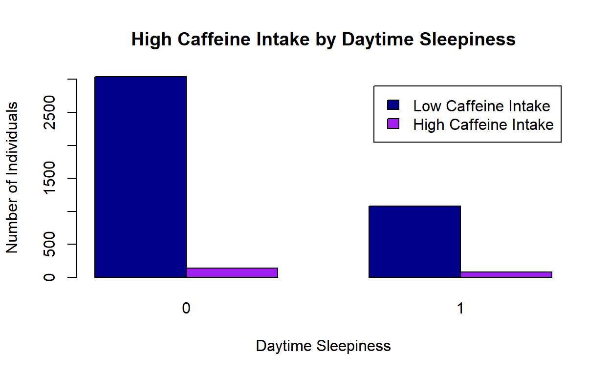
#dev.off()
Figure 2: Dperession and Daytime Sleepiness
#png("Barplot Depression.png")
counts <- table(unweighted_data$depress_cat, unweighted_data$day_sleep)
barplot(counts, main="Depression Category Distribution by Daytime Sleepiness",
        ylab = "Number of Individuals",
        xlab="Daytime Sleepiness", col=c("darkblue","purple","orange","yellow","lightblue"),
        legend = c("No Depression", "Mild Depression", "Moderate Depression", "Moderate/severe Depression", "Severe Depression"), beside=TRUE)
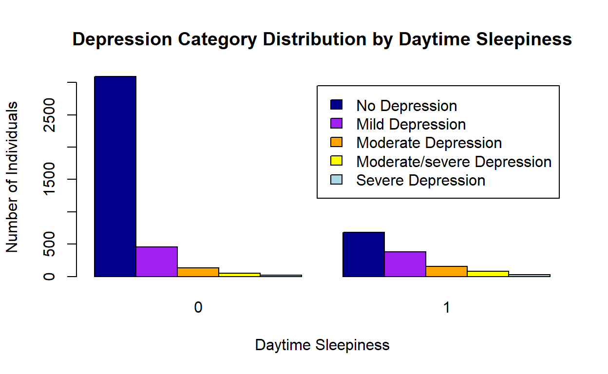
#dev.off()
Statistical Methods
Let’s develop a pipeline for our statistical analyses!
- Part a: Scatterplot matrices
- Part b: Fit weighted and unweighted SLRs
- Part c: Fit initial weighted and unweighted MLR model using all predictors
- Part d: Best subset model selection and human-selected model
- Part e. Compare model AICs and goodness of fit
- Part f: Check model: Analysis of Residuals
- Part f-1: Plot person residuals -vs- predicted values
- Part f-2: Boxplot and list outlier studentized residuals
- Part g: Check model: leverage boxplots
- Part h: Check model: influence
- Part h-1: Make boxplot and list outliers for influence
- Part h-2: Leverage -vs- residual squared (L-R) plot
- Part i: Sensitivity analysis: Re-fit without influential points
- Part j: Check for multi-collinearity using variance inflation factors
Part a: Scatterplot matrices
Using the ggpairs() function, which is nice for getting a quick scatterplot matrix plot
We must first created an unweighted dataset of those >=18.
Then we will make two separate scatterplot matrices. We must do this because if we make one matrix, it will be way too large and difficult to read. First we will make one of personal characteristics, and second, we will make one of lifestyle/behavioral characteristics.
unweighted_data <- filter(data, RIDAGEYR >=18)
#pdf("scatterplot_matrices_person.pdf")
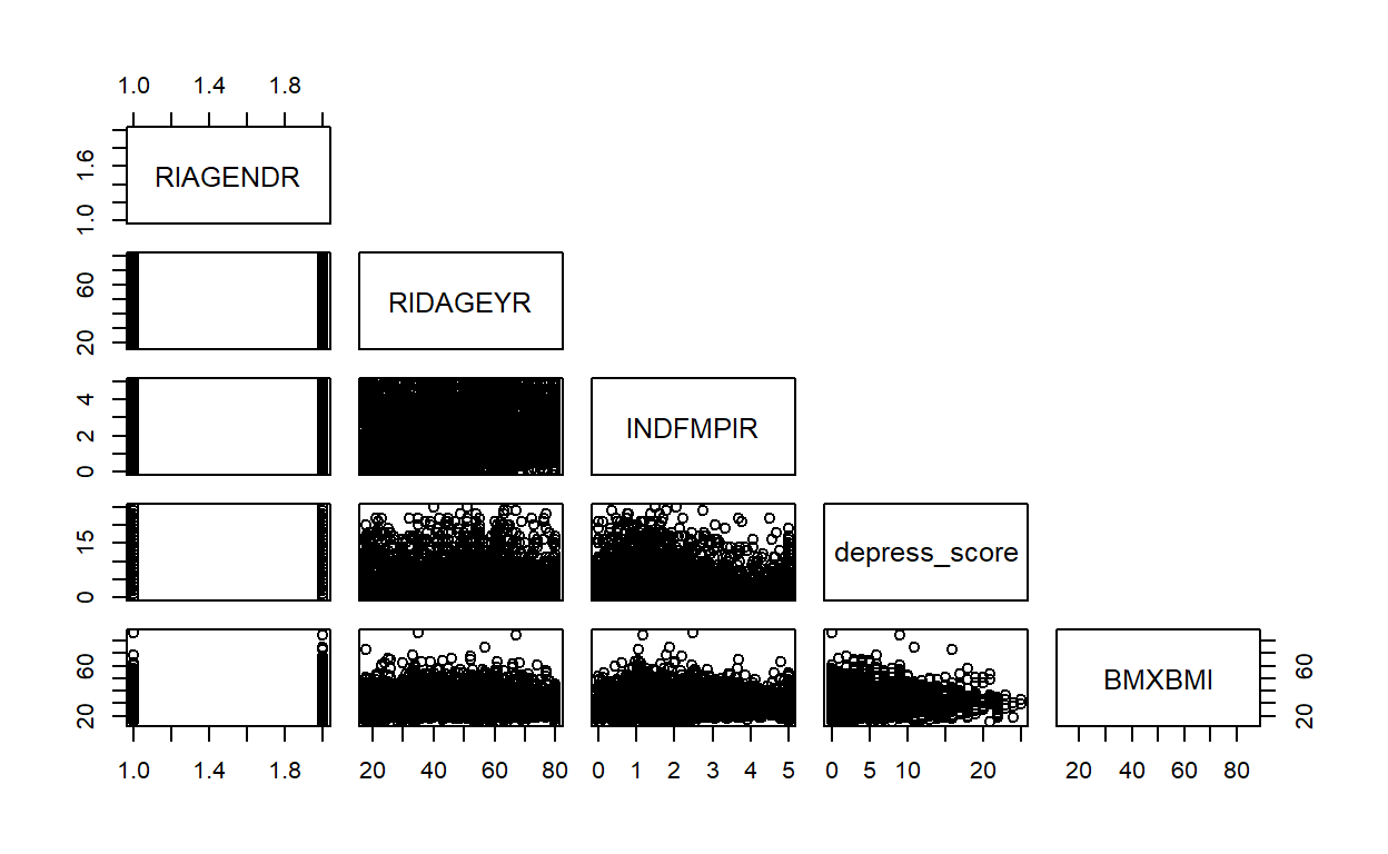
unweighted_data %>%
dplyr::select(RIAGENDR, RIDAGEYR, INDFMPIR,depress_score,BMXBMI) %>%
pairs(upper.panel=NULL)
#dev.off()
#pdf("scatterplot_matrices_behavior.pdf")
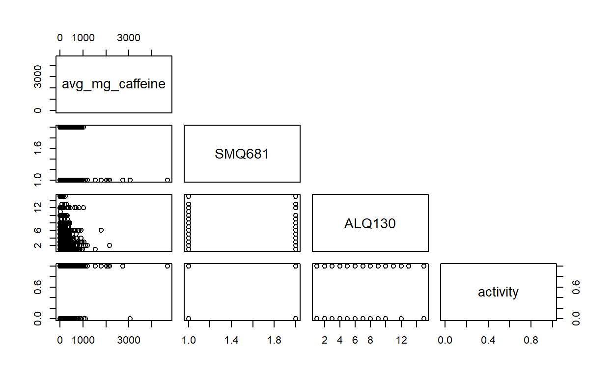
unweighted_data %>%
dplyr::select(avg_mg_caffeine,SMQ681,ALQ130,activity) %>%
pairs(upper.panel=NULL)
#dev.off()
There is no clear correlation between X’s.
Part b: Fit weighted and unweighted SLRs
Create a survey weight object
Fit the weighted univariate models and store the results. We are calculating the change in log prevalence odds of daytime sleepiness, our outcome, among levels of the “exposures”. Our exposures of interest are sex, age groups, income, smoking, race/ethnicity, any activity, high caffeine intake, BMI categories, heavy drinking, and ordinal depression scores. Log-binomial regression is used to estimate crude associations.
model_1w <- svyglm(day_sleep~RIAGENDR, design=NHANES, family=quasibinomial(link="log"))
model_2w <- svyglm(day_sleep~ageCat_18, design=NHANES, family=quasibinomial(link="log"))
model_3w <- svyglm(day_sleep~INDFMPIR, design=NHANES, family=quasibinomial(link="log"))
model_4w <- svyglm(day_sleep~SMQ681, design=NHANES, family=quasibinomial(link="log"))
model_5w <- svyglm(day_sleep~raceEthCat, design=NHANES, family=quasibinomial(link="log"))
model_6w <- svyglm(day_sleep~activity, design=NHANES, family=quasibinomial(link="log"))
model_7w <- svyglm(day_sleep~hi_caffeine, design=NHANES_MEC, family=quasibinomial(link="log"))
model_8w <- svyglm(day_sleep~BMI_cat, design=NHANES_MEC, family=quasibinomial(link="log"))
model_9w <- svyglm(day_sleep~heavy_drink2, design=NHANES, family=quasibinomial(link="log"))
model_10w <- svyglm(day_sleep~depress_cat, design=NHANES, family=quasibinomial(link="log"))
#exponentiated coefficients

exp(model_1w$coefficients)
(Intercept)    RIAGENDR
0.2048742 1.2206388 exp(model_2w$coefficients)
   (Intercept) ageCat_1840-59   ageCat_1860+
0.3183220 0.7924395 0.8044204 exp(model_3w$coefficients)
(Intercept)    INDFMPIR
0.3767510 0.9118087 exp(model_4w$coefficients)
(Intercept)      SMQ681
0.4012766 0.8151968 exp(model_5w$coefficients)
                (Intercept)          raceEthCatNH Black
                  0.3024167                   0.8091614
         raceEthCatNH Asian          raceEthCatHispanic
                  0.4615732                   0.7857788
raceEthCatNH Other/Multiple
1.2061075 exp(model_6w$coefficients)
(Intercept)    activity
0.2791679 0.9971760 exp(model_7w$coefficients)
(Intercept) hi_caffeine
0.2679387 1.4338962 exp(model_8w$coefficients)
       (Intercept) BMI_catunderweight  BMI_catoverweight
         0.2221463          1.2402763          1.0529336
      BMI_catobese
1.5503832 exp(model_9w$coefficients)
 (Intercept) heavy_drink2
0.2525171 1.2794627 exp(model_10w$coefficients)
  (Intercept) depress_cat.L depress_cat.Q depress_cat.C depress_cat^4
    0.4645206     2.2088022     0.5980783     1.2557422     0.9903052
# p-values
summary(model_1w)
Call:
svyglm(formula = day_sleep ~ RIAGENDR, design = NHANES, family = quasibinomial(link = "log"))

Survey design:
subset(NHANES_all, inAnalysis == 1)

Coefficients:
            Estimate Std. Error t value Pr(>|t|)
(Intercept) -1.58536    0.15227 -10.412 5.65e-08 ***
RIAGENDR     0.19937    0.08474   2.353   0.0338 *
---
Signif. codes:  0 '***' 0.001 '**' 0.01 '*' 0.05 '.' 0.1 ' ' 1

(Dispersion parameter for quasibinomial family taken to be 1.000171)

Number of Fisher Scoring iterations: 6summary(model_2w)
Call:
svyglm(formula = day_sleep ~ ageCat_18, design = NHANES, family = quasibinomial(link = "log"))

Survey design:
subset(NHANES_all, inAnalysis == 1)

Coefficients:
               Estimate Std. Error t value Pr(>|t|)
(Intercept)    -1.14469    0.05047 -22.680 7.73e-12 ***
ageCat_1840-59 -0.23264    0.06337  -3.671  0.00282 **
ageCat_1860+   -0.21763    0.07092  -3.069  0.00897 **
---
Signif. codes:  0 '***' 0.001 '**' 0.01 '*' 0.05 '.' 0.1 ' ' 1

(Dispersion parameter for quasibinomial family taken to be 1.000171)

Number of Fisher Scoring iterations: 6summary(model_3w)
Call:
svyglm(formula = day_sleep ~ INDFMPIR, design = NHANES, family = quasibinomial(link = "log"))

Survey design:
subset(NHANES_all, inAnalysis == 1)

Coefficients:
            Estimate Std. Error t value Pr(>|t|)
(Intercept) -0.97617    0.08189 -11.920 1.02e-08 ***
INDFMPIR    -0.09233    0.01919  -4.811 0.000277 ***
---
Signif. codes:  0 '***' 0.001 '**' 0.01 '*' 0.05 '.' 0.1 ' ' 1

(Dispersion parameter for quasibinomial family taken to be 1.026985)

Number of Fisher Scoring iterations: 6summary(model_4w)
Call:
svyglm(formula = day_sleep ~ SMQ681, design = NHANES, family = quasibinomial(link = "log"))

Survey design:
subset(NHANES_all, inAnalysis == 1)

Coefficients:
            Estimate Std. Error t value Pr(>|t|)
(Intercept) -0.91310    0.12122  -7.532 2.74e-06 ***
SMQ681      -0.20433    0.05779  -3.535  0.00329 **
---
Signif. codes:  0 '***' 0.001 '**' 0.01 '*' 0.05 '.' 0.1 ' ' 1

(Dispersion parameter for quasibinomial family taken to be 1.0229)

Number of Fisher Scoring iterations: 6summary(model_5w)
Call:
svyglm(formula = day_sleep ~ raceEthCat, design = NHANES, family = quasibinomial(link = "log"))

Survey design:
subset(NHANES_all, inAnalysis == 1)

Coefficients:
                            Estimate Std. Error t value Pr(>|t|)
(Intercept)                 -1.19595    0.04884 -24.490 6.03e-11 ***
raceEthCatNH Black          -0.21176    0.07694  -2.752   0.0188 *
raceEthCatNH Asian          -0.77311    0.09487  -8.149 5.48e-06 ***
raceEthCatHispanic          -0.24108    0.10810  -2.230   0.0475 *
raceEthCatNH Other/Multiple  0.18740    0.13200   1.420   0.1834
---
Signif. codes:  0 '***' 0.001 '**' 0.01 '*' 0.05 '.' 0.1 ' ' 1

(Dispersion parameter for quasibinomial family taken to be 1.000171)

Number of Fisher Scoring iterations: 6summary(model_6w)
Call:
svyglm(formula = day_sleep ~ activity, design = NHANES, family = quasibinomial(link = "log"))

Survey design:
subset(NHANES_all, inAnalysis == 1)

Coefficients:
             Estimate Std. Error t value Pr(>|t|)
(Intercept) -1.275942   0.059430 -21.470  4.1e-12 ***
activity    -0.002828   0.068327  -0.041    0.968
---
Signif. codes:  0 '***' 0.001 '**' 0.01 '*' 0.05 '.' 0.1 ' ' 1

(Dispersion parameter for quasibinomial family taken to be 1.000872)

Number of Fisher Scoring iterations: 6summary(model_7w)
Call:
svyglm(formula = day_sleep ~ hi_caffeine, design = NHANES_MEC,
    family = quasibinomial(link = "log"))

Survey design:
subset(NHANES_all_MEC, inAnalysis == 1)

Coefficients:
            Estimate Std. Error t value Pr(>|t|)
(Intercept) -1.31700    0.03985 -33.050 1.09e-14 ***
hi_caffeine  0.36040    0.12757   2.825   0.0135 *
---
Signif. codes:  0 '***' 0.001 '**' 0.01 '*' 0.05 '.' 0.1 ' ' 1

(Dispersion parameter for quasibinomial family taken to be 1.104844)

Number of Fisher Scoring iterations: 6summary(model_8w)
Call:
svyglm(formula = day_sleep ~ BMI_cat, design = NHANES_MEC, family = quasibinomial(link = "log"))

Survey design:
subset(NHANES_all_MEC, inAnalysis == 1)

Coefficients:
                   Estimate Std. Error t value Pr(>|t|)
(Intercept)        -1.50442    0.07922 -18.991 2.55e-10 ***
BMI_catunderweight  0.21533    0.28243   0.762 0.460528
BMI_catoverweight   0.05158    0.13810   0.374 0.715285
BMI_catobese        0.43850    0.10153   4.319 0.000998 ***
---
Signif. codes:  0 '***' 0.001 '**' 0.01 '*' 0.05 '.' 0.1 ' ' 1

(Dispersion parameter for quasibinomial family taken to be 1.064164)

Number of Fisher Scoring iterations: 6summary(model_9w)
Call:
svyglm(formula = day_sleep ~ heavy_drink2, design = NHANES, family = quasibinomial(link = "log"))

Survey design:
subset(NHANES_all, inAnalysis == 1)

Coefficients:
             Estimate Std. Error t value Pr(>|t|)
(Intercept)  -1.37628    0.06028 -22.830 1.78e-12 ***
heavy_drink2  0.24644    0.05956   4.138  0.00101 **
---
Signif. codes:  0 '***' 0.001 '**' 0.01 '*' 0.05 '.' 0.1 ' ' 1

(Dispersion parameter for quasibinomial family taken to be 1.022591)

Number of Fisher Scoring iterations: 6summary(model_10w)
Call:
svyglm(formula = day_sleep ~ depress_cat, design = NHANES, family = quasibinomial(link = "log"))

Survey design:
subset(NHANES_all, inAnalysis == 1)

Coefficients:
               Estimate Std. Error t value Pr(>|t|)
(Intercept)   -0.766749   0.059637 -12.857 5.71e-08 ***
depress_cat.L  0.792450   0.105804   7.490 1.22e-05 ***
depress_cat.Q -0.514034   0.093152  -5.518 0.000181 ***
depress_cat.C  0.227727   0.075092   3.033 0.011395 *
depress_cat^4 -0.009742   0.075368  -0.129 0.899485
---
Signif. codes:  0 '***' 0.001 '**' 0.01 '*' 0.05 '.' 0.1 ' ' 1

(Dispersion parameter for quasibinomial family taken to be 1.026629)

Number of Fisher Scoring iterations: 6 2.5 % 97.5 %
(Intercept) 0.1477932 0.2840011
RIAGENDR 1.0177826 1.4639265 2.5 % 97.5 %
(Intercept) 0.2854385 0.3549939
ageCat_1840-59 0.6910498 0.9087050
ageCat_1860+ 0.6901471 0.9376148 2.5 % 97.5 %
(Intercept) 0.3160633 0.4490912
INDFMPIR 0.8750411 0.9501211 2.5 % 97.5 %
(Intercept) 0.3094055 0.5204269
SMQ681 0.7201610 0.9227741 2.5 % 97.5 %
(Intercept) 0.2715973 0.3367333
raceEthCatNH Black 0.6831119 0.9584698
raceEthCatNH Asian 0.3745883 0.5687572
raceEthCatHispanic 0.6193948 0.9968574
raceEthCatNH Other/Multiple 0.9020059 1.6127337 2.5 % 97.5 %
(Intercept) 0.2457586 0.317119
activity 0.8612465 1.154559 2.5 % 97.5 %
(Intercept) 0.2459903 0.2918454
hi_caffeine 1.0906713 1.8851310 2.5 % 97.5 %
(Intercept) 0.1869307 0.2639961
BMI_catunderweight 0.6702992 2.2949234
BMI_catoverweight 0.7793414 1.4225720
BMI_catobese 1.2427144 1.9342241 2.5 % 97.5 %
(Intercept) 0.2218905 0.2873711
heavy_drink2 1.1260268 1.4538061 2.5 % 97.5 %
(Intercept) 0.4073797 0.5296763
depress_cat.L 1.7499334 2.7879959
depress_cat.Q 0.4872101 0.7341754
depress_cat.C 1.0644425 1.4814219
depress_cat^4 0.8389312 1.1689926Let’s also look at the univariate associations in unweighted models. We expect a change in the standard errors. It will not be as representative of the US population. We will store the results and diplay them in a table in the results section.
# fit the unweighted models and store the results

model_1u <- glm(day_sleep~RIAGENDR, family=binomial(link="log"), data = unweighted_data)
model_2u <- glm(day_sleep~ageCat_18, family=binomial(link="log"), data = unweighted_data)
model_3u <- glm(day_sleep~INDFMPIR, family=binomial(link="log"), data = unweighted_data)
model_4u <- glm(day_sleep~SMQ681, family=binomial(link="log"), data = unweighted_data)
model_5u <- glm(day_sleep~raceEthCat, family=binomial(link="log"), data = unweighted_data)
model_6u <- glm(day_sleep~activity, family=binomial(link="log"), data = unweighted_data)
model_7u <- glm(day_sleep~hi_caffeine, family=binomial(link="log"), data = unweighted_data)
model_8u <- glm(day_sleep~BMI_cat, family=binomial(link="log"), data = unweighted_data)
model_9u <- glm(day_sleep~heavy_drink2, family=binomial(link="log"), data = unweighted_data)
model_10u <- glm(day_sleep~depress_cat, family=binomial(link="log"), data = unweighted_data)
Part c: Fit initial MLR using all predictors
Multivariable Poisson regression with robust standard errors will be used to estimate adjusted prevalence ratios. Unweighted multivariable candidate models were selected in 4 ways:
- Including all predictors
- Best subset selection
- a-priori selection based on literature and common knowledge
- Combination of a priori and best-subset
First, lets run the models with every predictor
Note: logit models failed to converge. Use poisson model. From the svy package: svyglm always returns ‘model-robust’ standard errors; the Horvitz-Thompson-type standard errors used everywhere in the survey package are a generalisation of the model-robust ‘sandwich’ estimators. In particular, a quasi-Poisson svyglm will return correct standard errors for relative risk regression models.
Using Exam weights (recommended):
MLR_1 <- svyglm(day_sleep~RIAGENDR+ INDFMPIR + SMQ681 + ageCat_18+
                           + raceEthCat + activity + hi_caffeine + BMI_cat +
                             heavy_drink2 + depress_cat, design=NHANES_MEC,
                           family=quasipoisson(link="log"))

summary(MLR_1, df.resid = degf(NHANES_MEC))
Call:
svyglm(formula = day_sleep ~ RIAGENDR + INDFMPIR + SMQ681 + ageCat_18 +
    +raceEthCat + activity + hi_caffeine + BMI_cat + heavy_drink2 +
    depress_cat, design = NHANES_MEC, family = quasipoisson(link = "log"))

Survey design:
subset(NHANES_all_MEC, inAnalysis == 1)

Coefficients:
                             Estimate Std. Error t value Pr(>|t|)
(Intercept)                 -1.082160   0.233512  -4.634 0.000324 ***
RIAGENDR                     0.121471   0.078823   1.541 0.144130
INDFMPIR                    -0.052522   0.019994  -2.627 0.019049 *
SMQ681                       0.095709   0.068990   1.387 0.185622
ageCat_1840-59              -0.226165   0.095069  -2.379 0.031076 *
ageCat_1860+                -0.238507   0.081341  -2.932 0.010300 *
raceEthCatNH Black          -0.238056   0.105131  -2.264 0.038800 *
raceEthCatNH Asian          -0.557554   0.173805  -3.208 0.005868 **
raceEthCatHispanic          -0.307914   0.099593  -3.092 0.007442 **
raceEthCatNH Other/Multiple  0.064766   0.159042   0.407 0.689595
activity                     0.026327   0.057780   0.456 0.655168
hi_caffeine                  0.226425   0.095594   2.369 0.031709 *
BMI_catunderweight          -0.062413   0.362150  -0.172 0.865473
BMI_catoverweight            0.105170   0.160207   0.656 0.521471
BMI_catobese                 0.380563   0.106197   3.584 0.002716 **
heavy_drink2                 0.058645   0.083379   0.703 0.492609
depress_cat.L                0.643917   0.102021   6.312 1.39e-05 ***
depress_cat.Q               -0.426273   0.084199  -5.063 0.000140 ***
depress_cat.C                0.239641   0.093666   2.558 0.021828 *
depress_cat^4               -0.005434   0.075550  -0.072 0.943615
---
Signif. codes:  0 '***' 0.001 '**' 0.01 '*' 0.05 '.' 0.1 ' ' 1

Zero or negative residual df; p-values not defined

(Dispersion parameter for quasipoisson family taken to be 0.8208122)

Number of Fisher Scoring iterations: 6
#linearHypothesis(MLR_1, "ageCat_1818-39=ageCat_1840-59")
#linearHypothesis(MLR_1, "ageCat_1818-39=ageCat_1860+")
exp(MLR_1$coefficients)
                (Intercept)                    RIAGENDR
                  0.3388629                   1.1291569
                   INDFMPIR                      SMQ681
                  0.9488333                   1.1004391
             ageCat_1840-59                ageCat_1860+
                  0.7975861                   0.7878033
         raceEthCatNH Black          raceEthCatNH Asian
                  0.7881582                   0.5726078
         raceEthCatHispanic raceEthCatNH Other/Multiple
                  0.7349785                   1.0669093
                   activity                 hi_caffeine
                  1.0266769                   1.2541089
         BMI_catunderweight           BMI_catoverweight
                  0.9394944                   1.1108992
               BMI_catobese                heavy_drink2
                  1.4631086                   1.0603987
              depress_cat.L               depress_cat.Q
                  1.9039230                   0.6529379
              depress_cat.C               depress_cat^4
                  1.2707934                   0.9945811
Using Interview weights
MLR_2 <- svyglm(day_sleep~RIAGENDR + ageCat_18 + INDFMPIR + SMQ681
                + raceEthCat + activity + hi_caffeine + BMI_cat +
                  heavy_drink2 + depress_cat, design=NHANES,
                family=quasipoisson(link="log"))

summary(MLR_2, df.resid = degf(NHANES))
Call:
svyglm(formula = day_sleep ~ RIAGENDR + ageCat_18 + INDFMPIR +
    SMQ681 + raceEthCat + activity + hi_caffeine + BMI_cat +
    heavy_drink2 + depress_cat, design = NHANES, family = quasipoisson(link = "log"))

Survey design:
subset(NHANES_all, inAnalysis == 1)

Coefficients:
                             Estimate Std. Error t value Pr(>|t|)
(Intercept)                 -1.089417   0.237501  -4.587 0.000356 ***
RIAGENDR                     0.125684   0.080332   1.565 0.138535
ageCat_1840-59              -0.226016   0.093995  -2.405 0.029561 *
ageCat_1860+                -0.252454   0.080819  -3.124 0.006972 **
INDFMPIR                    -0.052001   0.019399  -2.681 0.017113 *
SMQ681                       0.093046   0.069257   1.343 0.199087
raceEthCatNH Black          -0.239878   0.105846  -2.266 0.038658 *
raceEthCatNH Asian          -0.556917   0.176800  -3.150 0.006607 **
raceEthCatHispanic          -0.306654   0.098127  -3.125 0.006952 **
raceEthCatNH Other/Multiple  0.065960   0.164823   0.400 0.694660
activity                     0.039479   0.059561   0.663 0.517487
hi_caffeine                  0.235958   0.094373   2.500 0.024492 *
BMI_catunderweight          -0.097781   0.377249  -0.259 0.799009
BMI_catoverweight            0.107206   0.162556   0.660 0.519570
BMI_catobese                 0.380365   0.107844   3.527 0.003050 **
heavy_drink2                 0.052873   0.082232   0.643 0.529948
depress_cat.L                0.643541   0.105453   6.103 2.02e-05 ***
depress_cat.Q               -0.422803   0.083392  -5.070 0.000138 ***
depress_cat.C                0.250825   0.089710   2.796 0.013570 *
depress_cat^4                0.001431   0.076402   0.019 0.985299
---
Signif. codes:  0 '***' 0.001 '**' 0.01 '*' 0.05 '.' 0.1 ' ' 1

Zero or negative residual df; p-values not defined

(Dispersion parameter for quasipoisson family taken to be 0.7764147)

Number of Fisher Scoring iterations: 6exp(MLR_2$coefficients)
                (Intercept)                    RIAGENDR
                  0.3364125                   1.1339234
             ageCat_1840-59                ageCat_1860+
                  0.7977057                   0.7768921
                   INDFMPIR                      SMQ681
                  0.9493281                   1.0975126
         raceEthCatNH Black          raceEthCatNH Asian
                  0.7867238                   0.5729726
         raceEthCatHispanic raceEthCatNH Other/Multiple
                  0.7359049                   1.0681840
                   activity                 hi_caffeine
                  1.0402691                   1.2661215
         BMI_catunderweight           BMI_catoverweight
                  0.9068478                   1.1131640
               BMI_catobese                heavy_drink2
                  1.4628178                   1.0542955
              depress_cat.L               depress_cat.Q
                  1.9032081                   0.6552077
              depress_cat.C               depress_cat^4
                  1.2850850                   1.0014325
Un-weighted
MLR_3 <- glm(day_sleep~RIAGENDR + ageCat_18 + INDFMPIR + SMQ681
             + raceEthCat + activity + hi_caffeine + BMI_cat +
               heavy_drink2 + depress_cat, family=poisson(link="log"), data = unweighted_data)

summary(MLR_3)
Call:
glm(formula = day_sleep ~ RIAGENDR + ageCat_18 + INDFMPIR + SMQ681 +
    raceEthCat + activity + hi_caffeine + BMI_cat + heavy_drink2 +
    depress_cat, family = poisson(link = "log"), data = unweighted_data)

Deviance Residuals:
    Min       1Q   Median       3Q      Max
-1.3717  -0.6854  -0.5868   0.3796   1.7553

Coefficients:
                            Estimate Std. Error z value Pr(>|z|)
(Intercept)                 -0.80381    0.20016  -4.016 5.92e-05 ***
RIAGENDR                     0.06662    0.06524   1.021  0.30718
ageCat_1840-59              -0.18448    0.08036  -2.296  0.02169 *
ageCat_1860+                -0.19778    0.08158  -2.424  0.01534 *
INDFMPIR                    -0.03071    0.02143  -1.433  0.15184
SMQ681                       0.10030    0.08124   1.235  0.21696
raceEthCatNH Black          -0.34815    0.08526  -4.083 4.44e-05 ***
raceEthCatNH Asian          -0.64845    0.13840  -4.686 2.79e-06 ***
raceEthCatHispanic          -0.37725    0.08883  -4.247 2.17e-05 ***
raceEthCatNH Other/Multiple -0.13584    0.13158  -1.032  0.30192
activity                    -0.06755    0.07090  -0.953  0.34068
hi_caffeine                  0.11217    0.12508   0.897  0.36983
BMI_catunderweight          -0.26905    0.28795  -0.934  0.35012
BMI_catoverweight            0.08017    0.09485   0.845  0.39798
BMI_catobese                 0.23308    0.08521   2.735  0.00623 **
heavy_drink2                 0.02428    0.07038   0.345  0.73014
depress_cat.L                0.72063    0.15763   4.572 4.84e-06 ***
depress_cat.Q               -0.43440    0.14050  -3.092  0.00199 **
depress_cat.C                0.21783    0.12248   1.779  0.07531 .
depress_cat^4               -0.05760    0.10252  -0.562  0.57419
---
Signif. codes:  0 '***' 0.001 '**' 0.01 '*' 0.05 '.' 0.1 ' ' 1

(Dispersion parameter for poisson family taken to be 1)

    Null deviance: 2612.4  on 3678  degrees of freedom
Residual deviance: 2320.8  on 3659  degrees of freedom
  (2177 observations deleted due to missingness)
AIC: 4384.8

Number of Fisher Scoring iterations: 6coeftest(MLR_3, vcov = sandwich)
z test of coefficients:

                             Estimate Std. Error z value  Pr(>|z|)
(Intercept)                 -0.803810   0.155923 -5.1552 2.534e-07
RIAGENDR                     0.066625   0.052285  1.2743  0.202572
ageCat_1840-59              -0.184479   0.063186 -2.9196  0.003504
ageCat_1860+                -0.197776   0.065378 -3.0251  0.002485
INDFMPIR                    -0.030711   0.017555 -1.7494  0.080213
SMQ681                       0.100302   0.064105  1.5647  0.117662
raceEthCatNH Black          -0.348150   0.069915 -4.9796 6.370e-07
raceEthCatNH Asian          -0.648454   0.123021 -5.2711 1.356e-07
raceEthCatHispanic          -0.377252   0.071291 -5.2917 1.212e-07
raceEthCatNH Other/Multiple -0.135836   0.098084 -1.3849  0.166087
activity                    -0.067554   0.056518 -1.1952  0.231990
hi_caffeine                  0.112169   0.094040  1.1928  0.232956
BMI_catunderweight          -0.269051   0.228246 -1.1788  0.238488
BMI_catoverweight            0.080168   0.079409  1.0096  0.312710
BMI_catobese                 0.233082   0.070999  3.2829  0.001027
heavy_drink2                 0.024277   0.056023  0.4333  0.664765
depress_cat.L                0.720634   0.097246  7.4104 1.259e-13
depress_cat.Q               -0.434399   0.086629 -5.0145 5.318e-07
depress_cat.C                0.217833   0.075467  2.8864  0.003896
depress_cat^4               -0.057602   0.065414 -0.8806  0.378544

(Intercept)                 ***
RIAGENDR
ageCat_1840-59              **
ageCat_1860+                **
INDFMPIR                    .
SMQ681
raceEthCatNH Black          ***
raceEthCatNH Asian          ***
raceEthCatHispanic          ***
raceEthCatNH Other/Multiple
activity
hi_caffeine
BMI_catunderweight
BMI_catoverweight
BMI_catobese                **
heavy_drink2
depress_cat.L               ***
depress_cat.Q               ***
depress_cat.C               **
depress_cat^4
---
Signif. codes: 0 '***' 0.001 '**' 0.01 '*' 0.05 '.' 0.1 ' ' 1exp(MLR_3$coefficients)
                (Intercept)                    RIAGENDR
                  0.4476202                   1.0688942
             ageCat_1840-59                ageCat_1860+
                  0.8315377                   0.8205536
                   INDFMPIR                      SMQ681
                  0.9697560                   1.1055052
         raceEthCatNH Black          raceEthCatNH Asian
                  0.7059933                   0.5228535
         raceEthCatHispanic raceEthCatNH Other/Multiple
                  0.6857430                   0.8729861
                   activity                 hi_caffeine
                  0.9346777                   1.1187019
         BMI_catunderweight           BMI_catoverweight
                  0.7641043                   1.0834689
               BMI_catobese                heavy_drink2
                  1.2624850                   1.0245741
              depress_cat.L               depress_cat.Q
                  2.0557369                   0.6476537
              depress_cat.C               depress_cat^4
                  1.2433790                   0.9440252
The unweighted regression results are qualitatively the same as the weighted regression results. I I also am not able to easily perform regression diagnostics with the survey weighted glm, so I will proceed with the unweighted model 3 for simplicity. This is reasonable, since we are trying to observe risk factors to daytime sleepiness in our sample and are not trying to predict prevalence of these risk factors in the United States population.
Part d: selection of best model using AIC and a priori
Next, we will run our best subset AI model to select the most parsimonious predictors
We will also attempt best-subset model selection to ensure that we are not missing any potentially relevant variables in our a-priori models.
analytic_data <- na.omit(unweighted_data)

# can do this all at once with step function when done by AIC
model_0 <- glm(day_sleep ~ 1, data = analytic_data, family = poisson(link = "log"))    # start with null model
mod_final <- step(model_0, scope = ~ . + RIAGENDR + ageCat_18 + INDFMPIR-1 + SMQ681
                  + activity + hi_caffeine + BMI_cat + raceEthCat +
                    heavy_drink2 + depress_cat, family=poisson(link="log"),
                  data = analytic_data, direction = "forward", na.rm = TRUE)   # add terms one at a time using AIC
Start:  AIC=2514.33
day_sleep ~ 1

               Df Deviance    AIC
+ depress_cat   4   1198.9 2450.9
+ raceEthCat    4   1256.2 2508.2
+ INDFMPIR      1   1262.8 2508.8
+ BMI_cat       3   1262.0 2512.0
+ hi_caffeine   1   1267.4 2513.4
<none>              1270.3 2514.3
+ RIAGENDR      1   1269.2 2515.2
+ ageCat_18     2   1267.8 2515.8
+ heavy_drink2  1   1269.8 2515.8
+ SMQ681        1   1269.9 2515.9
+ activity      1   1270.2 2516.2

Step:  AIC=2450.89
day_sleep ~ depress_cat

               Df Deviance    AIC
+ raceEthCat    4   1187.4 2447.4
<none>              1198.9 2450.9
+ INDFMPIR      1   1197.1 2451.1
+ hi_caffeine   1   1197.8 2451.8
+ ageCat_18     2   1195.8 2451.8
+ RIAGENDR      1   1198.4 2452.4
+ BMI_cat       3   1194.5 2452.5
+ activity      1   1198.5 2452.5
+ SMQ681        1   1198.7 2452.7
+ heavy_drink2  1   1198.9 2452.9

Step:  AIC=2447.4
day_sleep ~ depress_cat + raceEthCat

               Df Deviance    AIC
+ ageCat_18     2   1183.2 2447.2
+ INDFMPIR      1   1185.3 2447.3
<none>              1187.4 2447.4
+ SMQ681        1   1186.8 2448.8
+ RIAGENDR      1   1187.1 2449.1
+ activity      1   1187.1 2449.1
+ hi_caffeine   1   1187.1 2449.1
+ heavy_drink2  1   1187.4 2449.4
+ BMI_cat       3   1183.4 2449.4

Step:  AIC=2447.2
day_sleep ~ depress_cat + raceEthCat + ageCat_18

               Df Deviance    AIC
<none>              1183.2 2447.2
+ INDFMPIR      1   1181.7 2447.7
+ SMQ681        1   1182.0 2448.0
+ BMI_cat       3   1178.4 2448.4
+ hi_caffeine   1   1182.7 2448.7
+ heavy_drink2  1   1183.0 2448.9
+ RIAGENDR      1   1183.0 2449.0
+ activity 1 1183.2 2449.2coeftest(mod_final, vcov. = sandwich)
z test of coefficients:

                             Estimate Std. Error z value  Pr(>|z|)
(Intercept)                 -0.482284   0.063935 -7.5433 4.581e-14
depress_cat.L                0.576384   0.129384  4.4548 8.396e-06
depress_cat.Q               -0.392328   0.115405 -3.3996 0.0006749
depress_cat.C                0.042799   0.092111  0.4646 0.6421856
depress_cat^4               -0.041453   0.074945 -0.5531 0.5801898
raceEthCatNH Black          -0.232862   0.083771 -2.7798 0.0054400
raceEthCatNH Asian          -0.448282   0.149246 -3.0036 0.0026677
raceEthCatHispanic          -0.277537   0.084456 -3.2862 0.0010156
raceEthCatNH Other/Multiple -0.150954   0.115582 -1.3060 0.1915424
ageCat_1840-59              -0.115274   0.071351 -1.6156 0.1061843
ageCat_1860+                -0.204843   0.079876 -2.5645 0.0103322

(Intercept)                 ***
depress_cat.L               ***
depress_cat.Q               ***
depress_cat.C
depress_cat^4
raceEthCatNH Black          **
raceEthCatNH Asian          **
raceEthCatHispanic          **
raceEthCatNH Other/Multiple
ageCat_1840-59
ageCat_1860+                *
---
Signif. codes: 0 '***' 0.001 '**' 0.01 '*' 0.05 '.' 0.1 ' ' 1summary(mod_final)
Call:
glm(formula = day_sleep ~ depress_cat + raceEthCat + ageCat_18,
    family = poisson(link = "log"), data = analytic_data)

Deviance Residuals:
    Min       1Q   Median       3Q      Max
-1.2781  -0.7799  -0.6942   0.6298   1.3459

Coefficients:
                            Estimate Std. Error z value Pr(>|z|)
(Intercept)                 -0.48228    0.09852  -4.895 9.81e-07 ***
depress_cat.L                0.57638    0.20265   2.844  0.00445 **
depress_cat.Q               -0.39233    0.18092  -2.169  0.03012 *
depress_cat.C                0.04280    0.14962   0.286  0.77484
depress_cat^4               -0.04145    0.12182  -0.340  0.73365
raceEthCatNH Black          -0.23286    0.10737  -2.169  0.03009 *
raceEthCatNH Asian          -0.44828    0.17580  -2.550  0.01077 *
raceEthCatHispanic          -0.27754    0.10892  -2.548  0.01083 *
raceEthCatNH Other/Multiple -0.15095    0.16024  -0.942  0.34617
ageCat_1840-59              -0.11527    0.09378  -1.229  0.21900
ageCat_1860+                -0.20484    0.10283  -1.992  0.04637 *
---
Signif. codes:  0 '***' 0.001 '**' 0.01 '*' 0.05 '.' 0.1 ' ' 1

(Dispersion parameter for poisson family taken to be 1)

    Null deviance: 1270.3  on 1726  degrees of freedom
Residual deviance: 1183.2  on 1716  degrees of freedom
AIC: 2447.2

Number of Fisher Scoring iterations: 5exp(mod_final$coefficients)
                (Intercept)               depress_cat.L
                  0.6173715                   1.7795910
              depress_cat.Q               depress_cat.C
                  0.6754827                   1.0437281
              depress_cat^4          raceEthCatNH Black
                  0.9593946                   0.7922631
         raceEthCatNH Asian          raceEthCatHispanic
                  0.6387248                   0.7576473
raceEthCatNH Other/Multiple              ageCat_1840-59
                  0.8598874                   0.8911220
               ageCat_1860+
                  0.8147754
We see the final model has depression category, race, and age as the most parsimonious predictors explaining daytime sleepiness in our sample
Now, let’s look at our a-priori models
Model using behavioral risk factors only (a priori)
mod_behav <- glm(day_sleep~SMQ681 + activity + hi_caffeine + heavy_drink2,
                     family=poisson(link="log"), data = unweighted_data)

#robust variance
coeftest(mod_behav, vcov = sandwich)
z test of coefficients:

              Estimate Std. Error z value  Pr(>|z|)
(Intercept)  -1.161584   0.122919 -9.4500 < 2.2e-16 ***
SMQ681       -0.085705   0.061396 -1.3959 0.1627367
activity     -0.109537   0.054449 -2.0117 0.0442484 *
hi_caffeine   0.320028   0.094668  3.3805 0.0007235 ***
heavy_drink2  0.149307   0.054189  2.7553 0.0058635 **
---
Signif. codes:  0 '***' 0.001 '**' 0.01 '*' 0.05 '.' 0.1 ' ' 1
#coefficents
exp(mod_behav$coefficients)
 (Intercept)       SMQ681     activity  hi_caffeine heavy_drink2
   0.3129899    0.9178654    0.8962488    1.3771665    1.1610298
Model combining a priori and best-subset selection
mod_final_behav <- glm(day_sleep~depress_cat + ageCat_18 + SMQ681 + activity + raceEthCat +
                          hi_caffeine + heavy_drink2, family=poisson(link="log"), data = unweighted_data)

summary(mod_final_behav)
Call:
glm(formula = day_sleep ~ depress_cat + ageCat_18 + SMQ681 +
    activity + raceEthCat + hi_caffeine + heavy_drink2, family = poisson(link = "log"),
    data = unweighted_data)

Deviance Residuals:
    Min       1Q   Median       3Q      Max
-1.3059  -0.6649  -0.5739   0.3749   1.7463

Coefficients:
                            Estimate Std. Error z value Pr(>|z|)
(Intercept)                 -0.60500    0.15997  -3.782 0.000156 ***
depress_cat.L                0.83543    0.13796   6.056 1.40e-09 ***
depress_cat.Q               -0.40609    0.12492  -3.251 0.001151 **
depress_cat.C                0.29800    0.11183   2.665 0.007706 **
depress_cat^4               -0.03835    0.09589  -0.400 0.689213
ageCat_1840-59              -0.18828    0.07594  -2.479 0.013167 *
ageCat_1860+                -0.21188    0.07645  -2.772 0.005579 **
SMQ681                       0.10213    0.07482   1.365 0.172250
activity                    -0.09067    0.06641  -1.365 0.172142
raceEthCatNH Black          -0.34672    0.08010  -4.328 1.50e-05 ***
raceEthCatNH Asian          -0.78766    0.13358  -5.897 3.71e-09 ***
raceEthCatHispanic          -0.36168    0.08289  -4.363 1.28e-05 ***
raceEthCatNH Other/Multiple -0.13766    0.12599  -1.093 0.274537
hi_caffeine                  0.11937    0.12200   0.978 0.327873
heavy_drink2                 0.03806    0.06676   0.570 0.568567
---
Signif. codes:  0 '***' 0.001 '**' 0.01 '*' 0.05 '.' 0.1 ' ' 1

(Dispersion parameter for poisson family taken to be 1)

    Null deviance: 2935.0  on 4164  degrees of freedom
Residual deviance: 2599.7  on 4150  degrees of freedom
  (1691 observations deleted due to missingness)
AIC: 4847.7

Number of Fisher Scoring iterations: 6coeftest(mod_final_behav, vcov = sandwich)
z test of coefficients:

                             Estimate Std. Error z value  Pr(>|z|)
(Intercept)                 -0.604997   0.121445 -4.9817 6.304e-07
depress_cat.L                0.835431   0.081969 10.1920 < 2.2e-16
depress_cat.Q               -0.406091   0.075380 -5.3872 7.156e-08
depress_cat.C                0.297997   0.071108  4.1908 2.780e-05
depress_cat^4               -0.038350   0.063182 -0.6070 0.5438610
ageCat_1840-59              -0.188282   0.060499 -3.1122 0.0018573
ageCat_1860+                -0.211885   0.061448 -3.4482 0.0005643
SMQ681                       0.102129   0.059907  1.7048 0.0882301
activity                    -0.090669   0.052991 -1.7110 0.0870746
raceEthCatNH Black          -0.346716   0.065189 -5.3187 1.045e-07
raceEthCatNH Asian          -0.787660   0.119233 -6.6061 3.946e-11
raceEthCatHispanic          -0.361676   0.067043 -5.3947 6.863e-08
raceEthCatNH Other/Multiple -0.137664   0.096014 -1.4338 0.1516323
hi_caffeine                  0.119369   0.092434  1.2914 0.1965662
heavy_drink2                 0.038062   0.053537  0.7110 0.4771127

(Intercept)                 ***
depress_cat.L               ***
depress_cat.Q               ***
depress_cat.C               ***
depress_cat^4
ageCat_1840-59              **
ageCat_1860+                ***
SMQ681                      .
activity                    .
raceEthCatNH Black          ***
raceEthCatNH Asian          ***
raceEthCatHispanic          ***
raceEthCatNH Other/Multiple
hi_caffeine
heavy_drink2
---
Signif. codes:  0 '***' 0.001 '**' 0.01 '*' 0.05 '.' 0.1 ' ' 1
Part e: AIC and Goodness of Fit (pearson’s chi-sq)
Now I will compare the fit of the models. I calculate deviance residuals since the models are poisson, not linear.
with(mod_final_behav, cbind(res.deviance = deviance, df = df.residual, p = pchisq(deviance, df.residual, lower.tail=FALSE)))
     res.deviance   df p
[1,] 2599.738 4150 1with(mod_final, cbind(res.deviance = deviance, df = df.residual,
p = pchisq(deviance, df.residual, lower.tail=FALSE)))
     res.deviance   df p
[1,] 1183.199 1716 1with(MLR_3, cbind(res.deviance = deviance, df = df.residual,
p = pchisq(deviance, df.residual, lower.tail=FALSE)))
     res.deviance   df p
[1,]     2320.764 3659 1
I calculate the fit of the models using Aikake’s Information Criterion, a measure of parsimony and model goodness of fit:
There was some lost data in the best subset regression since there was some missingness. Therefore, the AIC is not as great as it seems when run on the full dataset. Let’s try the best subset model on the full data:
Mod_bestsub <- glm(day_sleep ~ ageCat_18 + depress_cat + raceEthCat, data = unweighted_data, family = poisson(link = "log"))

AIC(Mod_bestsub)
[1] 5802.821We see in the analyses above that the model with the best fit is the model including all covariates. However, since the epidemiologic question is seeking to understand which the behavioral risk factors may be the most impactful on daytime sleepiness, we will proceed with the model including all behavioral covariates (ever smoking, moderate/high physical activity, race, high caffeine consumption, and heavy drinking) plus the covariates identified in the best-subset model (age and depression).
Part f: Model diagnostics
Model diagnostics that we will perform include residual versus fitted plots, Q-Q plots, leverage boxplots, residual boxplots and influential point boxplots.
Part f-1: Plot studentized residual -vs- predicted values
Calculate predicted values and residuals in weighted data - model w/ all covariates
fit_dat <- as.data.frame(MLR_1$fitted.values)
pearson_res_w <- residuals(MLR_1, type = "pearson")
fit_dat <- cbind(fit_dat, pearson_res_w)


fit_dat %>%
  ggplot(aes(x = MLR_1$fitted.values, y = pearson_res_w)) +
  geom_point() +
  geom_hline(yintercept = c(-2, 0, 2), col="red") +
  geom_smooth(method = lm) +
  labs(x = "Fitted values", y = "Pearson Residuals", title = "Residuals vs. Fitted values")
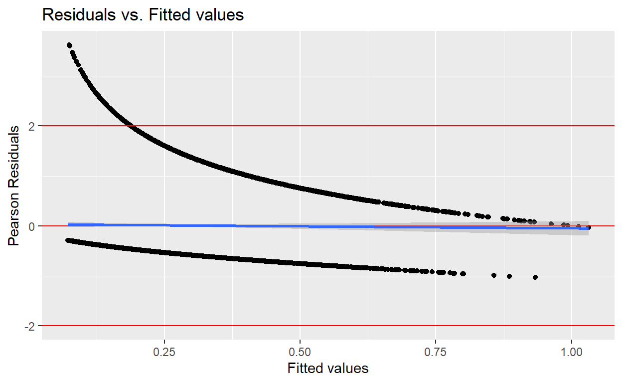
ggsave("pearson_resids_weighted.png", width = 6, height = 4, units = "in")
Calculate predicted values and residuals in unweighted data - model w/ all covariates
fit_dat2 <- as.data.frame(MLR_3$fitted.values)
pearson_res <- residuals(MLR_3, type = "pearson")
fit_dat2 <- cbind(fit_dat2, pearson_res)

fit_dat2 %>%
  ggplot(aes(x = MLR_3$fitted.values, y = pearson_res)) +
  geom_point() +
  geom_hline(yintercept = c(-2, 0, 2), col="red") +
  geom_smooth(method = lm) +
  labs(x = "Fitted values", y = "Pearson Residuals", title = "Residuals vs. Fitted values")
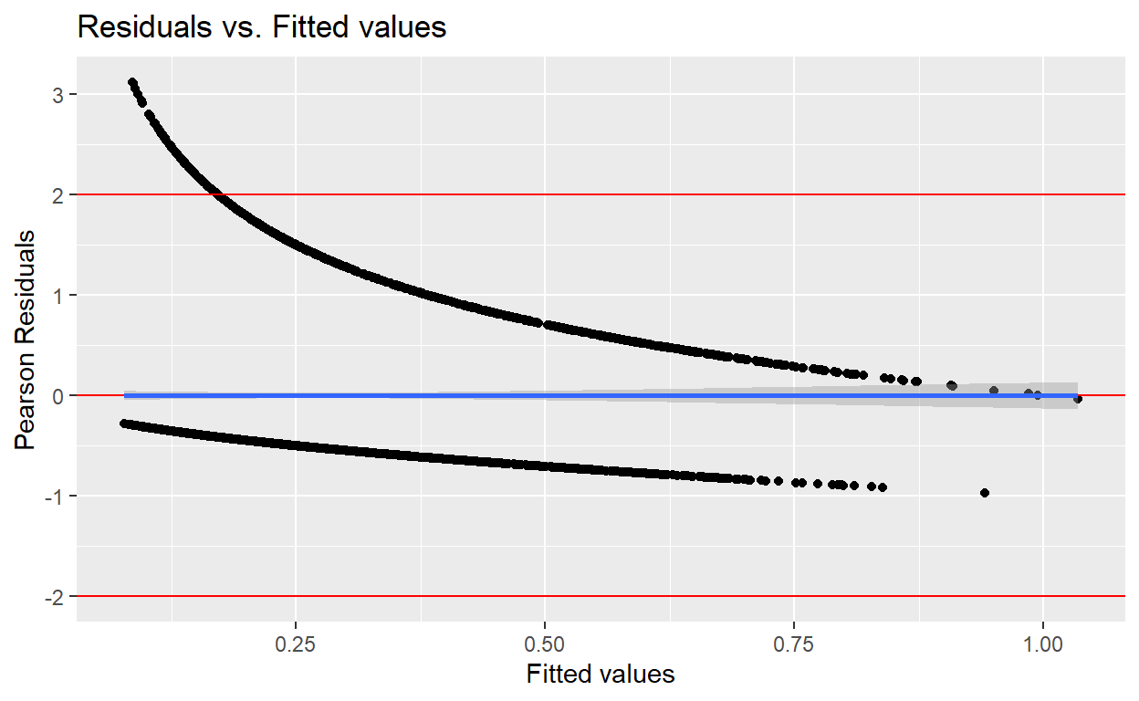
ggsave("pearson_resids_unweighted.png", width = 6, height = 4, units = "in")
The loess line is flat, which means there is no trend in the residuals. Equal variances/ linear assumption is met.
Calculate predicted values and residuals in unweighted final model
fit_dat_fin <- as.data.frame(mod_final_behav$fitted.values)
pearson_res_fin <- residuals(mod_final_behav, type = "pearson")
fit_dat_fin <- cbind(fit_dat_fin, pearson_res_fin)

fit_dat_fin %>%
  ggplot(aes(x = mod_final_behav$fitted.values, y = pearson_res_fin)) +
  geom_point() +
  geom_hline(yintercept = c(-2, 0, 2), col="red") +
  geom_smooth(method = lm) +
  labs(x = "Fitted values", y = "Pearson Residuals", title = "Residuals vs. Fitted values")
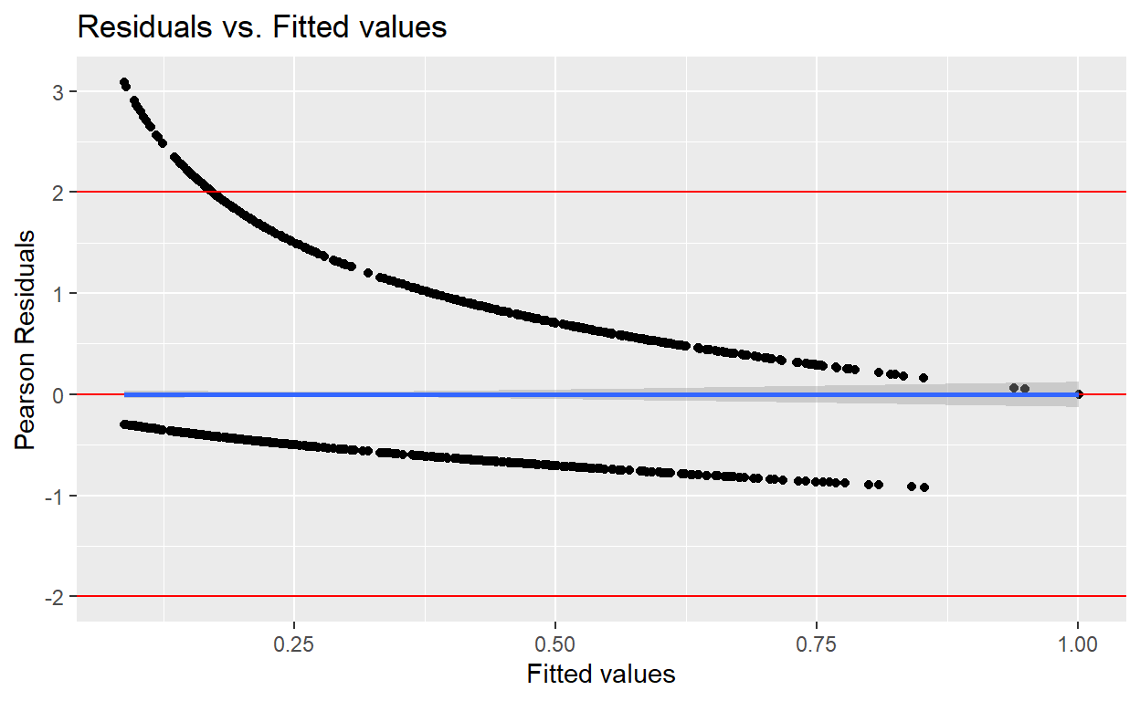
ggsave("pearson_resids_final_behave_model.png", width = 6, height = 4, units = "in")
Now, let’s create a Q-Q plot of deviance residuals for the final model and the model including all covariates
fit_dat_fin_apriori <- as.data.frame(mod_final_behav$fitted.values)
deviance_res_apriori <- residuals(mod_final_behav, type = "deviance")
fit_dat_fin_apriori <- cbind(fit_dat_fin_apriori, deviance_res_apriori)

fit_dat_fin_apriori %>%
  ggplot(aes(sample = deviance_res_apriori)) +
  geom_qq() +
  geom_qq_line() +
  labs(title = "Q-Q plot of deviance residuals")
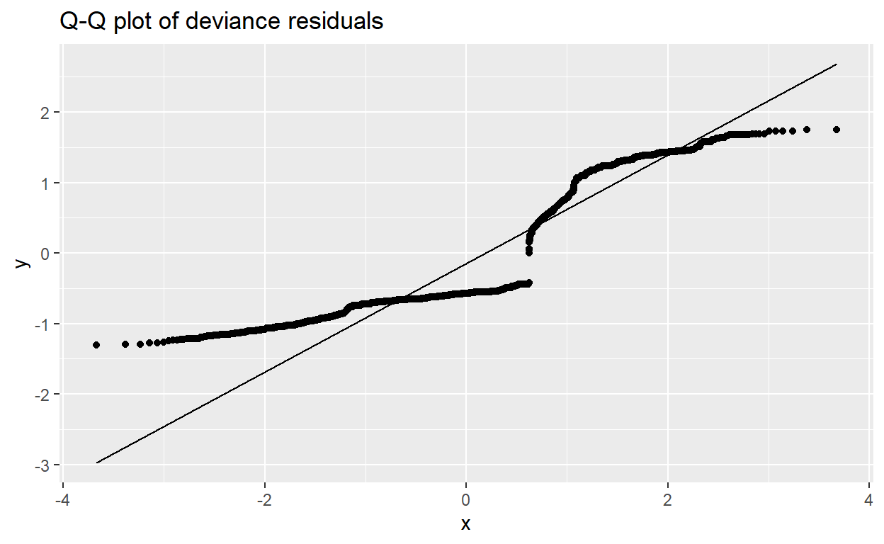
ggsave("Q-Q_final_behav_mod.png", width = 6, height = 4, units = "in")


fit_dat_fin_all <- as.data.frame(MLR_3$fitted.values)
deviance_res_fin <- residuals(MLR_3, type = "deviance")
fit_dat_fin_all <- cbind(fit_dat_fin_all, deviance_res_fin)

fit_dat_fin_all %>%
  ggplot(aes(sample = deviance_res_fin)) +
  geom_qq() +
  geom_qq_line() +
  labs(title = "Q-Q plot of deviance residuals")

ggsave("Q-Q_all_variables.png", width = 6, height = 4, units = "in")
Under the correct distribution of the response, we expect the points to align with the diagonal line. However, it is usual to have departures from the diagonal in the extremes other than in the center, even under normality. The graph is a little bit strange because we ran Poisson models, but the assumption is met.
Part f-2 : check outliers
Identify the outliers in the final a-priori models:
fit_dat_fin_apriori %>%
  ggplot() +
  geom_boxplot(aes(y = pearson_res_fin)) +
  labs(y="Pearson residuals", title="Boxplot of pearson residuals")
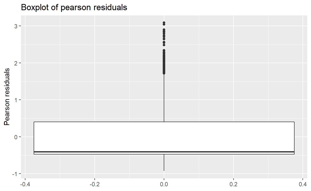
# Looking at the plot we can filter to see which observation is the outlier
outlier_list <- fit_dat_fin_apriori %>%
  filter(pearson_res_fin > 2.5)

glimpse(outlier_list)
Rows: 40
Columns: 2
$ `mod_final_behav$fitted.values` <dbl> 0.09910205, 0.09679036, 0.08~
$ deviance_res_apriori <dbl> 1.679707, 1.692335, 1.733906~nrow(outlier_list)
[1] 40#ggsave("outlier_residuals_apriori.png", width = 6, height = 4, units = "in")
Part g : check leverage
fit_dat_fin_apriori <- fit_dat_fin_apriori %>%
  mutate(lev = hatvalues(mod_final_behav))

# Boxplot of leverage values
fit_dat_fin_apriori %>%
  ggplot() +
  geom_boxplot(aes(y = lev)) +
  labs(y="Leverage values", title="Boxplot of leverages")
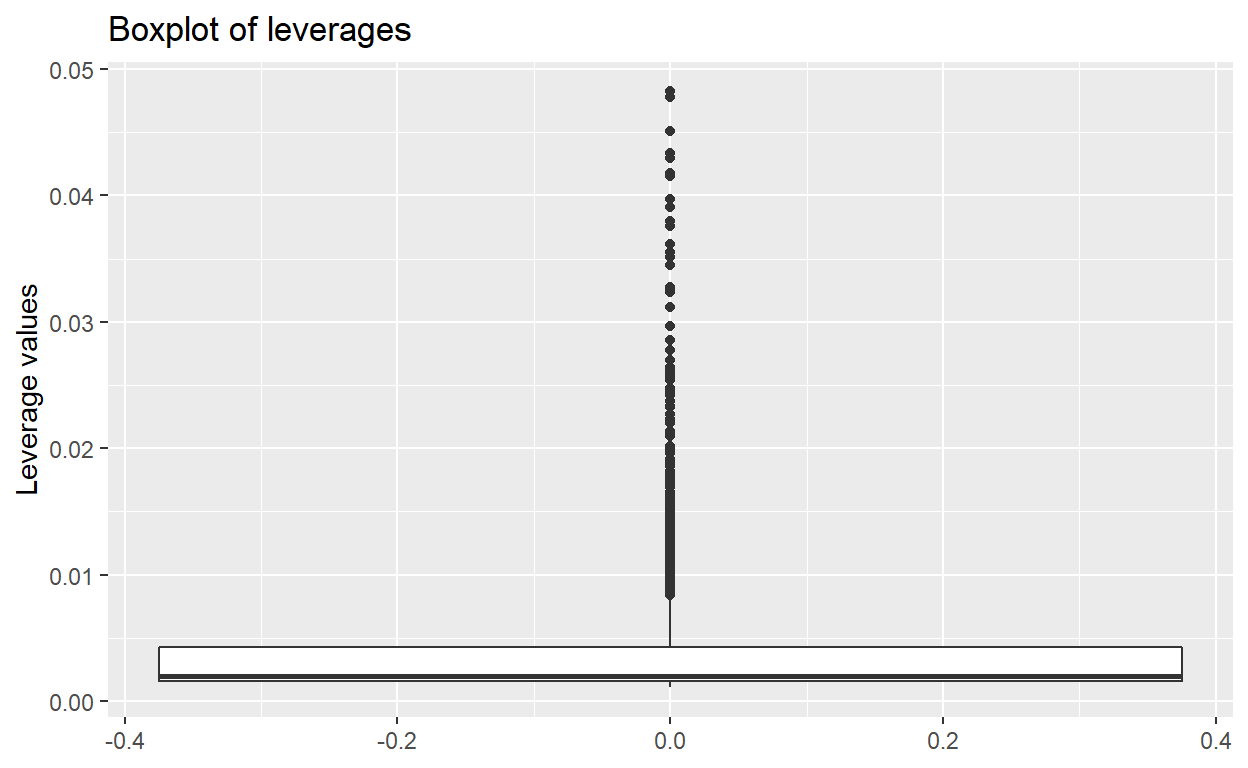
summary(fit_dat_fin_apriori$lev)
    Min.  1st Qu.   Median     Mean  3rd Qu.     Max.
0.001112 0.001548 0.001979 0.003601 0.004278 0.048211
lev_outliers <- 0.004278 + 1.5*(IQR(fit_dat_fin_apriori$lev))
list_lev_outliers <- fit_dat_fin_apriori %>%
filter(lev > lev_outliers)
glimpse(list_lev_outliers)
Rows: 336
Columns: 3
$ `mod_final_behav$fitted.values` <dbl> 0.5299878, 0.5505493, 0.6055~
$ deviance_res_apriori            <dbl> 0.5742631, 0.5429329, 0.4629~
$ lev <dbl> 0.010388046, 0.011440973, 0.~nrow(list_lev_outliers)
[1] 336#ggsave("Leverages_apriori.png", width = 6, height = 4, units = "in")
There are 336 leverage outliers!
Part h: Check model: influence
Part h-1: Make boxplot and list outliers for influence
# Calculate DFITS influence measure -- effect ith obs on overall fit
# Add them to data set
fit_dat_fin_apriori <- fit_dat_fin_apriori %>%
  mutate(dfits = dffits(mod_final_behav))

# Boxplot of dfits values
fit_dat_fin_apriori %>%
  ggplot() +
  geom_boxplot(aes(y = dfits)) +
  labs(y="DFITS values", title="Boxplot of DFIT values")
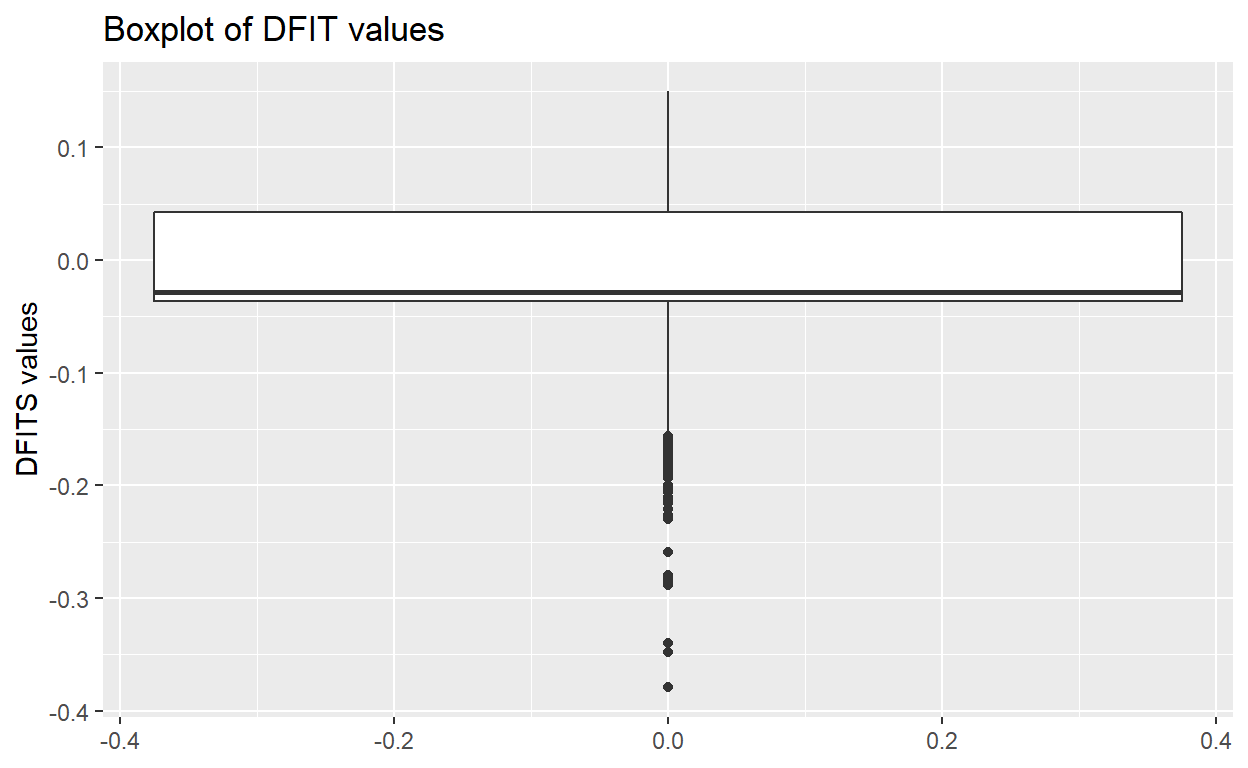
ggsave("dfits_apriori.png", width = 6, height = 4, units = "in")

# Look at outliers
influential_points <- fit_dat_fin_apriori %>%
  dplyr::select(dfits) %>%
  filter(dfits <= quantile(dfits, .25) - 1.5*IQR(dfits) |
           dfits >= quantile(dfits, .75) + 1.5*IQR(dfits)) %>%
  arrange(dfits)

glimpse(influential_points)
Rows: 56
Columns: 1
$ dfits <dbl> -0.3788205, -0.3478482, -0.3398676, -0.2887166, -0.285~nrow(influential_points)
[1] 56Part h-2: Leverage -vs- residual squared (L-R) plot
fit_dat_fin_apriori %>%
  ggplot(aes(x = pearson_res_fin^2, y = lev)) +
  geom_point() +
  geom_hline(yintercept = mean(fit_dat_fin_apriori$lev), col="red") +
  geom_vline(xintercept = mean(fit_dat_fin_apriori$pearson_res_fin^2), col="red") +
  labs(title="Leverage-Residual Plot")
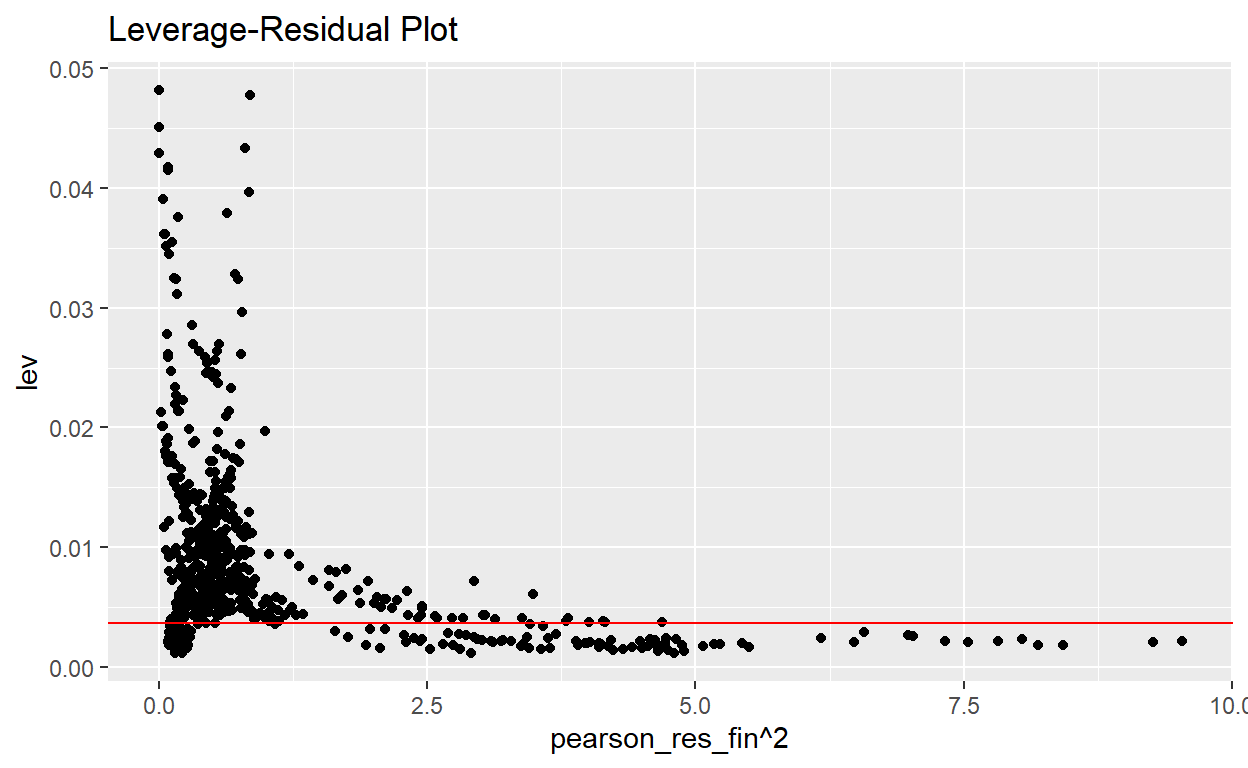
ggsave("L-R plot apriori.png", width = 6, height = 4, units = "in")
Part i: Sensitivity analysis: Re-fit without influential points
Sensitivity analysis conducted on the 8 most influential points:
Create new data set without influential points:
Fit the model without the influential points:
model_final_b_no_outliers <- glm(day_sleep~depress_cat + ageCat_18 + SMQ681 + activity +
                                   raceEthCat + hi_caffeine + heavy_drink2, family=poisson(link="log"), data = unweighted_data)

summary(model_final_b_no_outliers)
Call:
glm(formula = day_sleep ~ depress_cat + ageCat_18 + SMQ681 +
    activity + raceEthCat + hi_caffeine + heavy_drink2, family = poisson(link = "log"),
    data = unweighted_data)

Deviance Residuals:
    Min       1Q   Median       3Q      Max
-1.3059  -0.6649  -0.5739   0.3749   1.7463

Coefficients:
                            Estimate Std. Error z value Pr(>|z|)
(Intercept)                 -0.60500    0.15997  -3.782 0.000156 ***
depress_cat.L                0.83543    0.13796   6.056 1.40e-09 ***
depress_cat.Q               -0.40609    0.12492  -3.251 0.001151 **
depress_cat.C                0.29800    0.11183   2.665 0.007706 **
depress_cat^4               -0.03835    0.09589  -0.400 0.689213
ageCat_1840-59              -0.18828    0.07594  -2.479 0.013167 *
ageCat_1860+                -0.21188    0.07645  -2.772 0.005579 **
SMQ681                       0.10213    0.07482   1.365 0.172250
activity                    -0.09067    0.06641  -1.365 0.172142
raceEthCatNH Black          -0.34672    0.08010  -4.328 1.50e-05 ***
raceEthCatNH Asian          -0.78766    0.13358  -5.897 3.71e-09 ***
raceEthCatHispanic          -0.36168    0.08289  -4.363 1.28e-05 ***
raceEthCatNH Other/Multiple -0.13766    0.12599  -1.093 0.274537
hi_caffeine                  0.11937    0.12200   0.978 0.327873
heavy_drink2                 0.03806    0.06676   0.570 0.568567
---
Signif. codes:  0 '***' 0.001 '**' 0.01 '*' 0.05 '.' 0.1 ' ' 1

(Dispersion parameter for poisson family taken to be 1)

    Null deviance: 2935.0  on 4164  degrees of freedom
Residual deviance: 2599.7  on 4150  degrees of freedom
  (1691 observations deleted due to missingness)
AIC: 4847.7

Number of Fisher Scoring iterations: 6coeftest(mod_final_behav, vcov = sandwich)
z test of coefficients:

                             Estimate Std. Error z value  Pr(>|z|)
(Intercept)                 -0.604997   0.121445 -4.9817 6.304e-07
depress_cat.L                0.835431   0.081969 10.1920 < 2.2e-16
depress_cat.Q               -0.406091   0.075380 -5.3872 7.156e-08
depress_cat.C                0.297997   0.071108  4.1908 2.780e-05
depress_cat^4               -0.038350   0.063182 -0.6070 0.5438610
ageCat_1840-59              -0.188282   0.060499 -3.1122 0.0018573
ageCat_1860+                -0.211885   0.061448 -3.4482 0.0005643
SMQ681                       0.102129   0.059907  1.7048 0.0882301
activity                    -0.090669   0.052991 -1.7110 0.0870746
raceEthCatNH Black          -0.346716   0.065189 -5.3187 1.045e-07
raceEthCatNH Asian          -0.787660   0.119233 -6.6061 3.946e-11
raceEthCatHispanic          -0.361676   0.067043 -5.3947 6.863e-08
raceEthCatNH Other/Multiple -0.137664   0.096014 -1.4338 0.1516323
hi_caffeine                  0.119369   0.092434  1.2914 0.1965662
heavy_drink2                 0.038062   0.053537  0.7110 0.4771127

(Intercept)                 ***
depress_cat.L               ***
depress_cat.Q               ***
depress_cat.C               ***
depress_cat^4
ageCat_1840-59              **
ageCat_1860+                ***
SMQ681                      .
activity                    .
raceEthCatNH Black          ***
raceEthCatNH Asian          ***
raceEthCatHispanic          ***
raceEthCatNH Other/Multiple
hi_caffeine
heavy_drink2
---
Signif. codes: 0 '***' 0.001 '**' 0.01 '*' 0.05 '.' 0.1 ' ' 1exp(model_final_b_no_outliers$coefficients)
                (Intercept)               depress_cat.L
                  0.5460763                   2.3058075
              depress_cat.Q               depress_cat.C
                  0.6662495                   1.3471573
              depress_cat^4              ageCat_1840-59
                  0.9623758                   0.8283812
               ageCat_1860+                      SMQ681
                  0.8090580                   1.1075267
                   activity          raceEthCatNH Black
                  0.9133201                   0.7070058
         raceEthCatNH Asian          raceEthCatHispanic
                  0.4549079                   0.6965079
raceEthCatNH Other/Multiple                 hi_caffeine
                  0.8713918                   1.1267856
               heavy_drink2
1.0387961 exp(mod_final_behav$coefficients)
                (Intercept)               depress_cat.L
                  0.5460763                   2.3058075
              depress_cat.Q               depress_cat.C
                  0.6662495                   1.3471573
              depress_cat^4              ageCat_1840-59
                  0.9623758                   0.8283812
               ageCat_1860+                      SMQ681
                  0.8090580                   1.1075267
                   activity          raceEthCatNH Black
                  0.9133201                   0.7070058
         raceEthCatNH Asian          raceEthCatHispanic
                  0.4549079                   0.6965079
raceEthCatNH Other/Multiple                 hi_caffeine
                  0.8713918                   1.1267856
               heavy_drink2
                  1.0387961
Part j: Check variance inflation
vif(MLR_3) #check VIF of unweighted model with all risk factors
                 GVIF Df GVIF^(1/(2*Df))
RIAGENDR     1.059197  1        1.029173
ageCat_18    1.223982  2        1.051826
INDFMPIR     1.149586  1        1.072187
SMQ681       1.208305  1        1.099229
raceEthCat   1.225887  4        1.025785
activity     1.086719  1        1.042458
hi_caffeine  1.099705  1        1.048668
BMI_cat      1.114698  3        1.018262
heavy_drink2 1.160023  1        1.077044
depress_cat 1.126430 4 1.014993vif(mod_final) # check VIF of best subset model
                GVIF Df GVIF^(1/(2*Df))
depress_cat 1.021293  4        1.002637
raceEthCat  1.044998  4        1.005517
ageCat_18 1.042034 2 1.010347vif(mod_final_behav) # check VIF of a priori model
                 GVIF Df GVIF^(1/(2*Df))
depress_cat  1.060084  4        1.007320
ageCat_18    1.170830  2        1.040216
SMQ681       1.134808  1        1.065274
activity     1.056344  1        1.027786
raceEthCat   1.134959  4        1.015950
hi_caffeine  1.092136  1        1.045053
heavy_drink2 1.145752  1        1.070398
Results
unweighted_data %>%
  select(day_sleep, RIAGENDR, ageCat_18, INDFMPIR, SMQ681, raceEthCat, activity, hi_caffeine, BMI_cat, heavy_drink2, depress_cat) %>%
  tbl_uvregression(
    method = glm,
    y = day_sleep,
    method.args = list(family = binomial(link="log")),
    exponentiate = TRUE,
    pvalue_fun = ~style_pvalue(.x, digits = 2)
  ) %>%
  add_global_p() %>%  # add global p-value
  add_q() %>%         # adjusts global p-values for multiple testing
  bold_p() %>%        # bold p-values under a given threshold (default 0.05)
  bold_p(t = 0.10, q = TRUE) %>% # now bold q-values under the threshold of 0.10
  modify_caption("Crude Table") %>%
  bold_labels()
| Characteristic | N | RR1 | 95% CI1 | p-value | q-value2 |
|---|---|---|---|---|---|
| RIAGENDR | 5856 | 1.20 | 1.10, 1.31 | <0.001 | <0.001 |
| ageCat_18 | 5856 | <0.001 | 0.001 | ||
| 18-39 | — | — | |||
| 40-59 | 0.82 | 0.74, 0.92 | |||
| 60+ | 0.87 | 0.78, 0.96 | |||
| INDFMPIR | 5021 | 0.92 | 0.89, 0.95 | <0.001 | <0.001 |
| SMQ681 | 5132 | 0.85 | 0.76, 0.94 | 0.002 | 0.003 |
| raceEthCat | 5856 | <0.001 | <0.001 | ||
| NH White | — | — | |||
| NH Black | 0.68 | 0.61, 0.76 | |||
| NH Asian | 0.42 | 0.35, 0.49 | |||
| Hispanic | 0.67 | 0.60, 0.75 | |||
| NH Other/Multiple | 0.92 | 0.76, 1.09 | |||
| activity | 5849 | 0.95 | 0.87, 1.05 | 0.31 | 0.31 |
| hi_caffeine | 4339 | 1.41 | 1.16, 1.67 | <0.001 | 0.001 |
| BMI_cat | 5434 | <0.001 | <0.001 | ||
| normal | — | — | |||
| underweight | 1.07 | 0.71, 1.51 | |||
| overweight | 1.05 | 0.92, 1.20 | |||
| obese | 1.44 | 1.28, 1.62 | |||
| heavy_drink2 | 5120 | 1.23 | 1.12, 1.35 | <0.001 | <0.001 |
| depress_cat | 5068 | <0.001 | <0.001 | ||
| depress_cat.L | 2.42 | 2.02, 2.79 | |||
| depress_cat.Q | 0.61 | 0.52, 0.70 | |||
| depress_cat.C | 1.23 | 1.08, 1.40 | |||
| depress_cat^4 | 0.91 | 0.82, 1.02 | |||
|
1
RR = Relative Risk, CI = Confidence Interval
2
False discovery rate correction for multiple testing
|
|||||
Best subset model included race categories, age categories, and depression score categories as predictors. The final model was the model including behavioral variables selected a-priori, along with age and depression score which were identified through the AI model. This final model best suits the epidemiological question at hand: which risk factors are most important in the relationship with excessive daytime sleepiness, with a special emphasis on modifiable lifestyle factors?
- The predictors in the final model: age categories, race categories, depression score categories, current smoking, weekly moderate to vigorous activity, high caffeine intake, and heavy alcohol use
The dataset was large, so the model is still parsimonious with many predictors. All candidate models had Pearson’s Goodness of Fit p-values equal to 1, so all fit the data very well. None of the variables showed signs of collinearity for any of the candidate models.
Results from the final model:
mod_final_behav %>%
  tbl_regression(exponentiate = TRUE) %>%
  add_global_p() %>%  # add global p-value
  add_q() %>%         # adjusts global p-values for multiple testing
  bold_p() %>%        # bold p-values under a given threshold (default 0.05)
  bold_p(t = 0.10, q = TRUE) %>% # now bold q-values under the threshold of 0.10
  modify_caption("Final model") %>%
  bold_labels()
| Characteristic | IRR1 | 95% CI1 | p-value | q-value2 |
|---|---|---|---|---|
| depress_cat | <0.001 | <0.001 | ||
| depress_cat.L | 2.31 | 1.73, 2.98 | ||
| depress_cat.Q | 0.67 | 0.52, 0.84 | ||
| depress_cat.C | 1.35 | 1.08, 1.68 | ||
| depress_cat^4 | 0.96 | 0.80, 1.16 | ||
| ageCat_18 | 0.010 | 0.023 | ||
| 18-39 | — | — | ||
| 40-59 | 0.83 | 0.71, 0.96 | ||
| 60+ | 0.81 | 0.70, 0.94 | ||
| SMQ681 | 1.11 | 0.96, 1.28 | 0.2 | 0.2 |
| activity | 0.91 | 0.80, 1.04 | 0.2 | 0.2 |
| raceEthCat | <0.001 | <0.001 | ||
| NH White | — | — | ||
| NH Black | 0.71 | 0.60, 0.83 | ||
| NH Asian | 0.45 | 0.35, 0.59 | ||
| Hispanic | 0.70 | 0.59, 0.82 | ||
| NH Other/Multiple | 0.87 | 0.68, 1.11 | ||
| hi_caffeine | 1.13 | 0.88, 1.42 | 0.3 | 0.4 |
| heavy_drink2 | 1.04 | 0.91, 1.18 | 0.6 | 0.6 |
|
1
IRR = Incidence Rate Ratio, CI = Confidence Interval
2
False discovery rate correction for multiple testing
|
||||
- Belonging to older age groups (40-59 years & 60+ years) conferred a decreased risk of excessive daytime sleepiness when compared to a referent group of 18-39 years, contrary to what is expected based on the literature
- This may indicate that age-differential lifestyle factors confound the relationship between age and sleep quality.
- There was also an association in the opposite direction of to what is expected for race categories.
- When compared to white individuals, Hispanic, Asian, and Black individuals have a decreased risk of excessive daytime sleepiness
- Perhaps the relationship is confounded by social factors not accounted for in the study
- When compared to white individuals, Hispanic, Asian, and Black individuals have a decreased risk of excessive daytime sleepiness
- Associations with the most potential for intervention were mild and moderate to severe depression, caffeine intake, and obesity
- The direction of the association of depression score with excessive daytime sleepiness varied by severity, which may be due to low sample sizes in severity categories
- Some covariates previously presented as risk factors for poor sleep quality in the literature that were not replicated in this study were heavy alcohol use, current tobacco smoking, and participation in weekly moderate to vigorous physical activity
Conclusions and future directions
Conflicting results emphasize the need for more research is needed to uncover the links between age, race, alcohol use, tobacco smoking and exercise on sleep quality
High daily caffeine consumption is a modifiable risk factor that could play a role in causing excessive sleepiness during the day.
Based on these results and the results of previous research, it may be clinically advisable to address sleep hygiene in people with depression and obesity to prevent future morbidity and mortality.